Spatial accessibility and interaction through networks

In spatial data science, we use spatial graphs to reflect the degree of spatial interaction between observations. You already know how to represent interaction based on contiguity, distance or spatial regimes. However, in many contexts (notably urban ones), interaction follows spatially restricted movement patterns, such as those along street networks. In this session, we will cover movement through the streets as well as movement by public transport.

import datetime

import geopandas as gpd
import matplotlib.pyplot as plt
import numpy as np
import pandarm
import r5py
import shapely

from libpysal import graph, kernels

We start with the data on census areas in Prague, as we did in the last session. The dataset contains relatively granular spatial units with information about the population living in each, based on 2021 data.

prague = gpd.read_file(
    "https://martinfleischmann.net/sds/spatial_graphs/data/zsj_prague_2021.gpkg"
)
1prague = prague.set_index("NAZ_ZSJ")
prague.explore()

1: Use the name of the census area as an index. This will propagate to the graph itself.

Make this Notebook Trusted to load map: File -> Trust Notebook

Walking through the streets

First, we will rely on the pandarm package to model interactions reflecting movement (walking, driving and biking) through the streets.

All parts of the analysis here require you to build a routable network. While you can do this manually from sets of nodes and edges (with edge weights), the most common approach is to rely on the street network defined by OpenStreetMap. Given a GeoDataFrame, pandarm can fetch the data and construct such a network itself using pandarm.Network.from_gdf, as shown below. However, this uses the Overpass API, which is currently struggling to keep up with demand and block bots. To avoid additional requests, the code below was used to download, construct and save the network to an HDF5 file suitable for multi-component data like this.

network = pandarm.Network.from_gdf(prague, network_type="walk")
network.save_hdf5("data/prague_walk.h5")

We can load the saved file directly with pandarm. Download the prague_walk.h5 file and put it in the data folder (or change the path below).

network = pandarm.Network.from_hdf5("data/prague_walk.h5")

Generating contraction hierarchies with 4 threads.
Setting CH node vector of size 164176
Setting CH edge vector of size 456078
Range graph removed 461464 edges of 912156
. 10% . 20% . 30% . 40% . 50% . 60% . 70% . 80% . 90% . 100%

The network is, in principle, composed of two GeoDataFrames: one capturing edges (streets) and another capturing nodes (intersections).

Edges:

network.edges_df.head()

	from	to	length	geometry
0	172535	1484997498	5.828261	LINESTRING (-749800.809 -1044400.729, -749801....
1	247759	4323267352	87.174122	LINESTRING (-743581.867 -1042063.787, -743583....
2	247775	29049613	11.789723	LINESTRING (-740978.974 -1041297.258, -740967....
3	249170	661939051	87.366678	LINESTRING (-728417.277 -1040692.002, -728470....
4	249741	1278345642	21.446707	LINESTRING (-733664.919 -1042110.925, -733686....

Nodes:

network.nodes_df.head()

	x	y	geometry
osmid
172535	-749800.809475	-1.044401e+06	POINT (-749800.809 -1044400.729)
247759	-743581.866620	-1.042064e+06	POINT (-743581.867 -1042063.787)
247775	-740978.974083	-1.041297e+06	POINT (-740978.974 -1041297.258)
249170	-728417.277403	-1.040692e+06	POINT (-728417.277 -1040692.002)
249741	-733664.919088	-1.042111e+06	POINT (-733664.919 -1042110.925)

Nodes have a special role in pandarm.Network, as the analysis outcome is typically linked to node geometry, as we’ll see below.

The second dataset used in this session captures locations of public and private schools across Prague and comes from GeoPortalPraha.cz. Read the data and familiarise yourself with it.

schools = gpd.read_file(
    'https://martinfleischmann.net/sds/spatial_networks/data/schools.zip'
)
schools.head()

	NAZEV_ZAR	ULICE	CPOP	COR	PISM_COR	ADRESA_ZAR	KOD_TYPU	TYP_TXT	KAPACITA	POCET_ZAKU	DRUH_UAP	POSKYT	ID_POSKYT	ZRIZOVATEL	TYP_UAP	ZDROJ_POV	KAPACITA_R	geometry
0	Gymnázium prof. Jana Patočky, Praha 1, Jindřiš...	Jindřišská	966	36	NaN	JINDŘIŠSKÁ 966/36	C00	Střední škola	660	594	1	HMP-SMS	384	2	01_03	1	640	POINT (-742166.95 -1043426.68)
1	Akademické gymnázium a Jazyková škola s právem...	Štěpánská	614	22	NaN	ŠTĚPÁNSKÁ 614/22	F20	Jazyková škola s právem státní jazykové zkou	955	0	1	HMP-SMS	384	2	01_06	0	0	POINT (-742652.34 -1044042.59)
2	Akademické gymnázium a Jazyková škola s právem...	Štěpánská	614	22	NaN	ŠTĚPÁNSKÁ 614/22	C00	Střední škola	550	456	1	HMP-SMS	384	2	01_03	1	480	POINT (-742652.34 -1044042.59)
3	Gymnázium, Praha 2, Botičská 1	Botičská	424	1	NaN	BOTIČSKÁ 424/1	C00	Střední škola	435	407	1	HMP-SMS	384	2	01_03	1	416	POINT (-743295.29 -1045007.59)
4	Hotelová škola, Praha 10, Vršovická 43	Vršovická	564	43	NaN	VRŠOVICKÁ 564/43	C00	Střední škola	640	542	1	HMP-SMS	384	2	01_03	1	600	POINT (-740473.28 -1045615.24)

To work with the school locations within the network, we need to assign them to the network using the set_pois (set Points of Interest) method.

network.set_pois(
1    category="schools",
2    maxdist=2000,
3    maxitems=5,
4    x_col=schools.geometry.x,
    y_col=schools.geometry.y,
)

1: Define a name for this category of PoIs. You will use it later when referring to this point set.
2: Define the maximum distance we’ll later use in the search. pandarm will use it to avoid expensive computation beyond this threshold.
3: Define the maximum number of nearest items we will try to find later. Again, this is to optimise performance.
4: Pass the locations as arrays of X and Y coordinates. Note that these need to use the same CRS as the network.

Nearest POIs

Using this, you can find the distances to the nearest schools. At most, you can find the distances to the five nearest schools specified above.

nearest_schools = network.nearest_pois(
1    distance=2000,
    category="schools", 
2    num_pois=5,
)
nearest_schools.head()

1: Define the maximum search distance. The algorithm does not look beyond it.
2: Define the number of nearest PoIs to find.

	1	2	3	4	5
osmid
172535	1039.590942	1199.173950	1199.173950	1201.621948	1549.717041
247759	1023.289001	1141.755005	1141.755005	1141.755005	1289.784058
247775	526.362976	526.362976	526.362976	579.656982	579.656982
249170	1961.771973	2000.000000	2000.000000	2000.000000	2000.000000
249741	332.203003	368.191986	447.686005	544.693970	544.693970

The distance is measured from every node in the network and can be linked back to the nodes_df. That allows you to easily visualise the outcome: a map of the distance to the nearest school (of any kind) when walking along the street network.

ax = network.nodes_df.plot(nearest_schools[1], markersize=.01, legend=True)
ax.set_axis_off()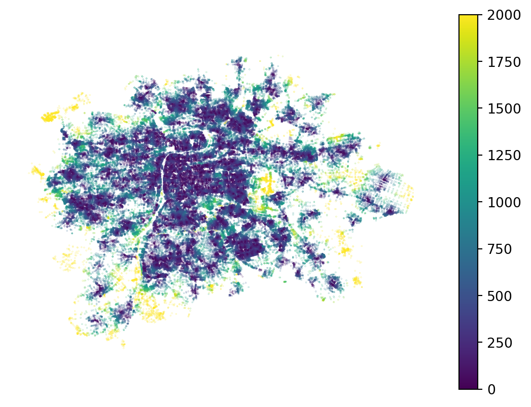

Distance to the nearest school from every intersection in Prague

For a better illustration, let’s use only a subset of specific schools. Filter out 'Základní umělecká škola', which are art schools.

art_school = schools.query("TYP_TXT == 'Základní umělecká škola'")
network.set_pois(
    category="art_school", 
1    maxdist=5000,
    maxitems=1,
    x_col=art_school.geometry.x, 
    y_col=art_school.geometry.y,
)

1: This pointset is sparser, so we might look further to find the nearest one.

Get the distances to the nearest art school. This time, also fetch the ID of the PoI, not just the distance.

nearest_art_school = network.nearest_pois(
    distance=5000, 
    category="art_school", 
    include_poi_ids=True,
)
nearest_art_school.head()

	1	poi1
osmid
172535	2096.083008	1125.0
247759	1669.810059	918.0
247775	1006.700012	179.0
249170	2404.993896	184.0
249741	4221.897949	164.0

The resulting DataFrame now contains two columns: the first captures the distance, and the second captures the ID of the nearest school. This ID is an integer position, not the index.

ax = art_school.plot(markersize=1, color='orange', zorder=2)
network.nodes_df.plot(
    nearest_art_school[1], markersize=.01, legend=True, ax=ax,
)
ax.set_axis_off()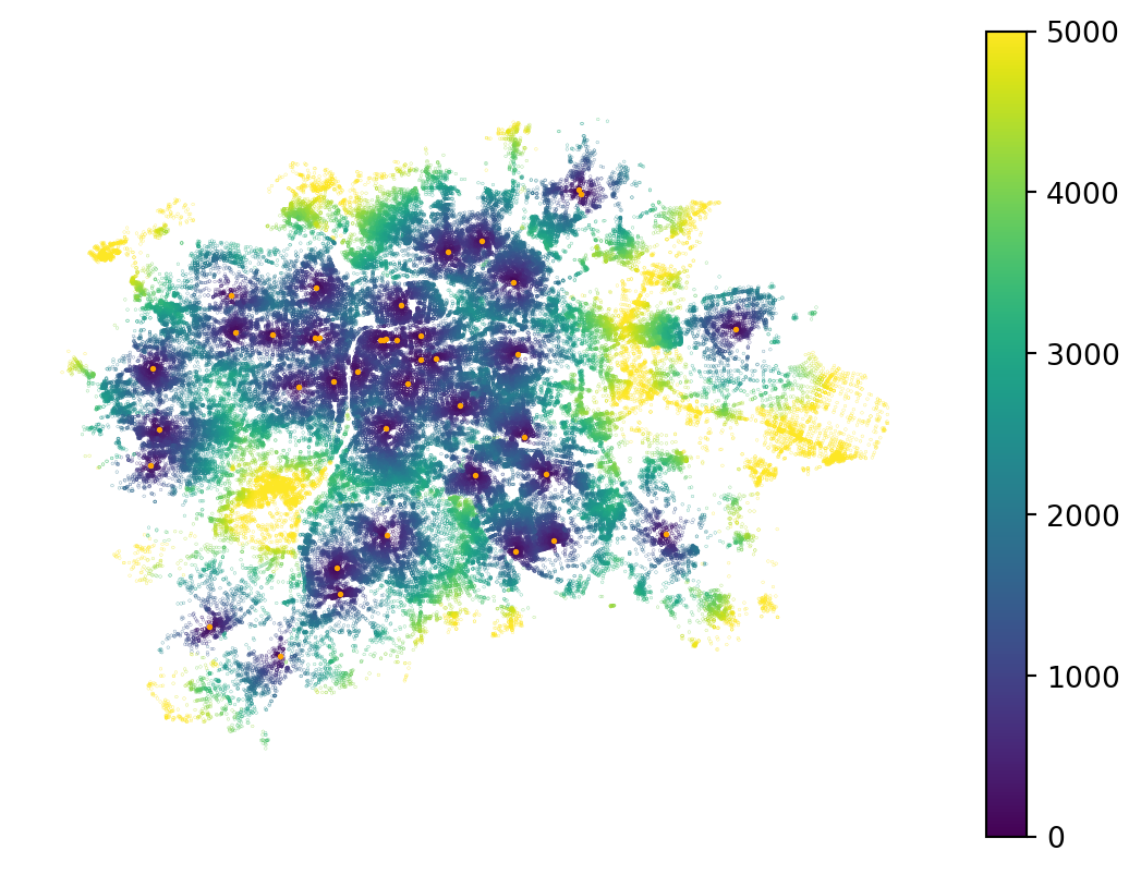

Distance to the nearest art school from every intersection in Prague

The ID column can be used to allocate nodes to the nearest school, as shown in the map below.

ax = art_school.plot(markersize=1, color='black', zorder=2)
network.nodes_df.plot(
    nearest_art_school["poi1"], markersize=.01, categorical=True, cmap="Spectral", ax=ax,
)
ax.set_axis_off()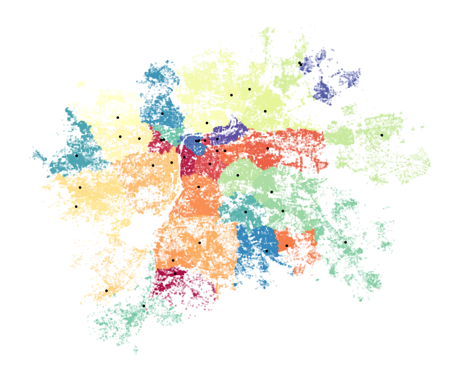

Intersections coloured by the nearest art school

This is, in principle, a Voronoi tessellation based on distance along the street network rather than typical Euclidean distance.

Isochrones

Since we have started allocating space to locations based on distance, let’s stick with this for a bit and explore isochrones. An isochrone delineates an area reachable via the network within a set time or distance. pandarm can help us define isochrones relatively easily (though we need to do some manual coding).

We’re going to generate isochrones reflecting an approximate 15-minute walking distance (~1200 metres) from each art school. To do so, we first need to identify the node in the network nearest to each art school, as the analysis is tied to existing nodes.

art_schoool_nodes = network.get_node_ids(
    art_school.geometry.x, 
    art_school.geometry.y,
)
art_schoool_nodes.head()

146     3306782858
149    10015367098
159    12157708905
160       25870382
161     5367208974
Name: node_id, dtype: int64

The resulting series gives us the ID of the node used to represent the approximate location of each art school. With this, you can find all other nodes in the specified range, which represents an isochrone.

isochrones = network.nodes_in_range(art_schoool_nodes, radius=1200)
isochrones

	source	destination	length
0	3306782858	3306782858	0.000000
1	3306782858	8278444953	3.376000
2	3306782858	3306785062	13.095000
3	3306782858	11833291704	57.842999
4	3306782858	5156403647	93.928001
...	...	...	...
70206	1026341251	29403434	1198.568970
70207	1026341251	21311322	1199.249023
70208	1026341251	12123917427	1199.676025
70209	1026341251	9083768815	1199.739990
70210	1026341251	4764026998	1199.937012

70211 rows × 3 columns

The output DataFrame is not the most user-friendly, but you can see that the source column contains repeated IDs of source nodes, along with all other nodes within the radius and the exact distance to them. Getting the isochrones as polygons is then a simple GeoPandas operation.

isochrones_poly = (
1    network.nodes_df.loc[isochrones["destination"]]
2    .dissolve(isochrones["source"].values)
3    .concave_hull(ratio=0.2)
)
isochrones_poly.head()

1: Get a node geometry per each destination.
2: Dissolve nodes to a single MultiPoint based on the source ID.
3: Draw concave hull around each MultiPoint to get the isochrone.

25870382     POLYGON ((-745679.337 -1042158.172, -745667.60...
25871906     POLYGON ((-747518.959 -1042144.518, -747518.45...
245500078    POLYGON ((-752310.617 -1047299.699, -752317.04...
257892802    POLYGON ((-743154.973 -1049828.186, -743106.66...
333793544    POLYGON ((-737570.236 -1042379.089, -737565.59...
dtype: geometry

You can now explore the outcome.

m = isochrones_poly.explore()
art_school.explore(m=m, color='red')

Make this Notebook Trusted to load map: File -> Trust Notebook

If that is of interest, you can further analyse and dissect the nodes forming the isochrones, as each has a distance. For example, you can peel off outer nodes to form smaller isochrones without recomputing the routes.

ax = network.nodes_df.loc[isochrones["destination"]].plot(isochrones['length'].values, markersize=.1, legend=True)
ax.set_axis_off()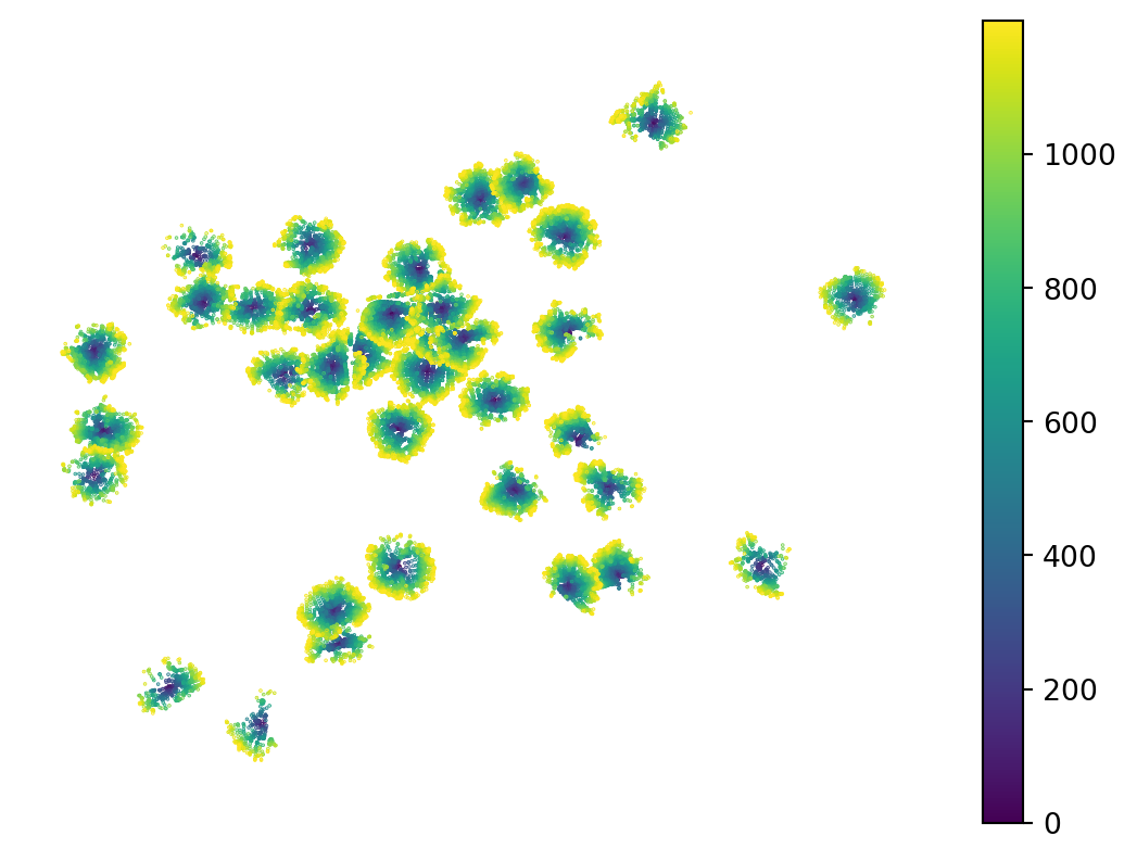

Distance to individual intersections forming the isochrone

Network-based aggregations

pandarm is also well suited for data aggregation along the network. This can capture accessible population, accessible school capacity or similar measures. Our school dataset contains information about school capacity in the KAPACITA column, so we can try to understand how capacity affects access.

We also have population information linked to census output areas, so we can ask how school capacity compares with the local population.

First, we need to assign variables to the network. Since we cannot add additional nodes to the network, we find the nearest existing node to each point with a value and assign the values to those nodes.

1art_node_ids = network.get_node_ids(art_school.geometry.x, art_school.geometry.y)
2pop_node_ids = network.get_node_ids(prague.centroid.x, prague.centroid.y)

3network.set(art_node_ids, variable=art_school["KAPACITA"], name="art_school_capacity")
4network.set(pop_node_ids, variable=prague["n_people"], name="population")

1: Get the ID of the nearest node in the network per each art school.
2: Get the ID of the node nearest to the centroid of each census area.
3: Assign art school capacity onto the identified nodes.
4: Assign population counts onto the identified nodes.

We are interested in the number of places in art schools within an accessible range per 1,000 people. By accessible, we mean approximately 30 minutes of walking, as people are more willing to walk further for specialised needs like this one. However, the further away a school is, the less willing people are to make the trip. We can therefore start by allocating accessible population to each node as a distance-weighted sum.

accessible_population = network.aggregate(
1    distance=2400,
2    func="sum",
3    decay="linear",
4    name="population",
)
accessible_population.head()

1: 2400 meters is approximately 30 minutes walking.
2: Specify the aggregation function as "sum".
3: Define linear decay so that locations further away count less.
4: Define the name of the variable we’re aggregating here.

osmid
172535     8569.827312
247759    12938.982047
247775    24497.160258
249170      795.958168
249741    12361.801134
dtype: float64

This aggregation results in a spatial distribution of accessible population that highlights areas of high population density, but is relatively smooth.

ax = network.nodes_df.plot(accessible_population, markersize=.01, legend=True)
ax.set_axis_off()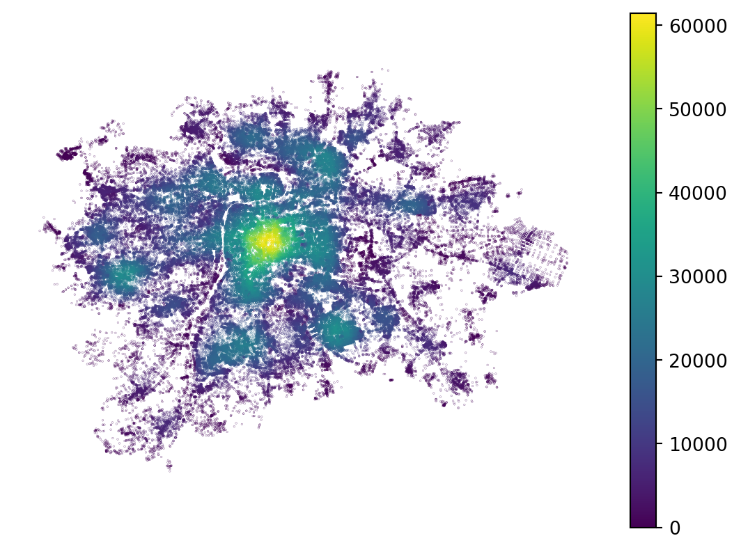

Accessible population within 2.5km along the street network

We can now do the same aggregation for the capacity of art schools, again using linear decay to account for the difference in willingness to walk as distance increases.

accessible_capacity = network.aggregate(
    distance=2400, 
    func="sum", 
    decay="linear", 
    name="art_school_capacity",
)

The accessible capacity then takes into account the locations of art schools, their individual capacities and the ability to reach them via the street network.

ax = art_school.plot(color='red', zorder=2, markersize=2)
ax = network.nodes_df.plot(accessible_capacity, markersize=.01, legend=True, ax=ax)
ax.set_axis_off()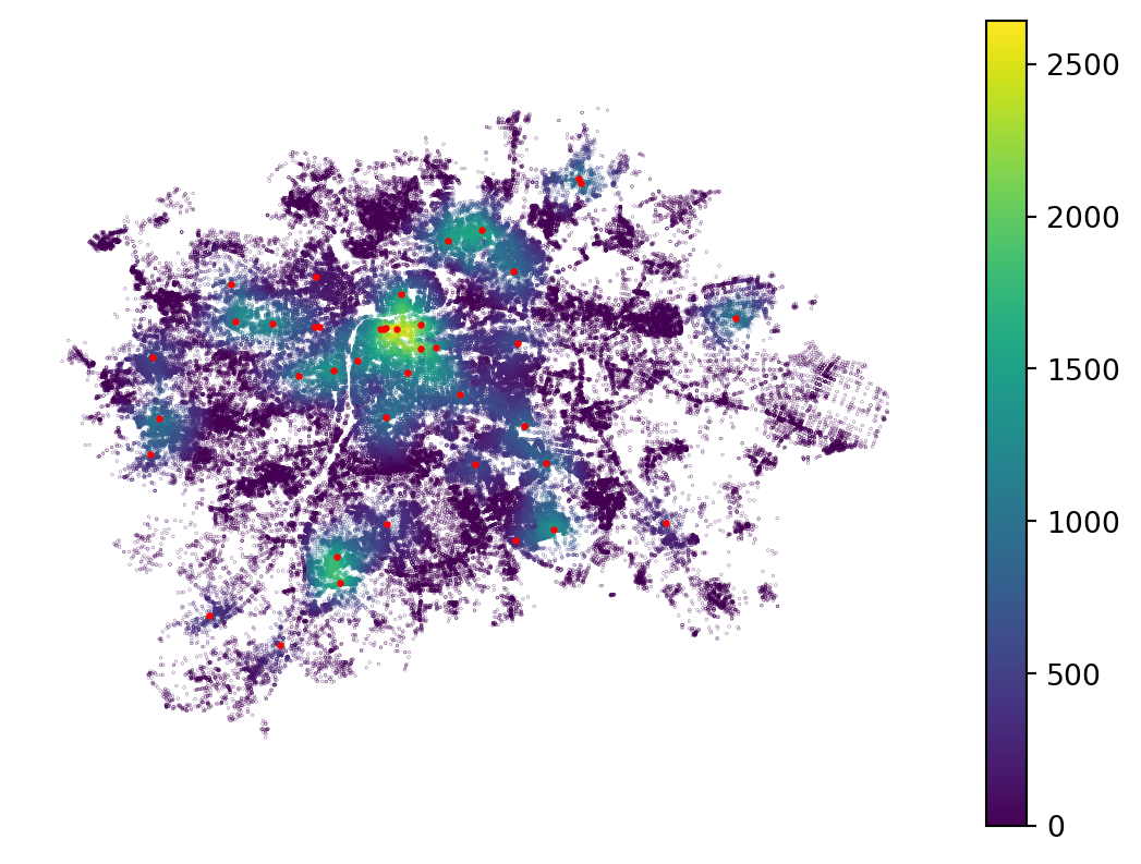

Accessible art school capacity within 2.5km along the street network

Now, we can simply normalise the accessible capacity by the accessible population to get an approximation of general art school accessibility.

normalised_capacity = (
    accessible_capacity / accessible_population
1).replace(np.inf, np.nan) * 1000

1: Dividing by zero results in infinity. Replace infinity with missing value. Multiplying by 1000 to get spots per 1000 inhabitants.

The results show hotspots of higher accessibility and coldspots of lower accessibility, with some peripheral locations indicating high accessibility. Those schools are quite likely serving a wider suburban region.

ax = art_school.plot(color='red', zorder=2, markersize=2)
network.nodes_df.plot(normalised_capacity, markersize=.01, legend=True, vmax=100, ax=ax)
ax.set_axis_off()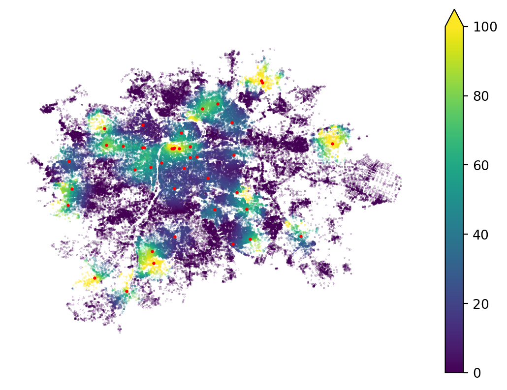

Population within 2.4km along the street network

Keep in mind that this example is an oversimplification, as people will often travel across the city using public transport, which significantly changes the perception of distance, as we will explore below.

Network interaction graphs

The idea of accessibility from one place to another through the street network can be translated into spatial weights encoding spatial interaction. libpysal has a built-in method to derive such weights from a provided pandarm network.

# this needs new libpysal
travel_cost_graph = graph.Graph.build_travel_cost(
1    prague.centroid,
2    network=network,
3    threshold=2400,
4    kernel="bisquare",
)
travel_cost_graph

1: Points to be snapped to network nodes.
2: The network to use to extract the distances.
3: Maximum distance within which two observations are considered neighbours.
4: A kernel that translates the raw network distance into a weight.

<Graph of 953 nodes and 21119 nonzero edges (8 components, 0 isolates) indexed by
 ['Běchovice', 'Nová Dubeč', 'Benice', 'Březiněves', 'Dolní Černošice', ...]>

The resulting Graph can be used like any other, for example, to derive a spatial lag.

lagged_population = travel_cost_graph.lag(prague["n_people"])
prague.explore(lagged_population)

Make this Notebook Trusted to load map: File -> Trust Notebook

Additional information

pandarm is a fork of another package named pandana, which was abandoned for years (but is now in maintenance mode). pandarm contains some additional functionality, but resources that refer to pandana also apply to pandarm. Simply replace pandana in the code with pandarm.

For more details, you can check the documentation for pandarm and pandana, and the chapter on Accessibility from Eli Knaap’s book Urban Analysis & Spatial Science.

Multi-modal movement

Up until now, we have assumed movement through the street network on foot. However, urban environments are often served by dense public transport networks, some of which run on streets and some of which do not. To provide a more realistic estimate of accessibility and network-based interaction, we shall combine different modes of transport and make full use of public transport. To do so, we need data capturing public transport schedules in a format called the General Transit Feed Specification (GTFS). This contains information about routes, stops, schedules, transfers, agencies running individual routes and other aspects of public transport systems. For Prague, you can get this information for two weeks ahead.

pandarm cannot model multimodal movement, but we can use another tool: r5py. It works similarly to pandarm by creating a network object first. In addition to the GTFS data, you need to provide a local extract from OpenStreetMap for r5py to use as its street network representation for routing.

transport_network = r5py.TransportNetwork(
1    osm_pbf="https://martinfleischmann.net/sds/spatial_networks/data/praha-261020.osm.pbf",
    gtfs=["https://martinfleischmann.net/sds/spatial_networks/data/PID_GTFS.zip"],
2    allow_errors=True,
)

1: An osm.pbf file can be downloaded from Geofabrik. The file used here was downloaded from there.
2: Prague’s GTFS data apparently has some issues with missing stop names. We can ignore them.

Isochrones

As with pandarm, we can delineate isochrones as areas accessible within a given time from one or more origins. The two packages work a bit differently, so their APIs do not match. Nevertheless, the concepts are similar. In r5py, generating isochrones is easier, as there is a dedicated method for doing so: r5py.Isochrones.

Let’s try to define isochrones around art schools in Prague as we did before, this time using public transport information.

1art_school['id'] = art_school.NAZEV_ZAR

isochrones = r5py.Isochrones(
    transport_network,
2    origins=art_school,
3    departure=datetime.datetime(2026, 10, 22, 10, 30),
4    isochrones=[5, 10, 15],
)
isochrones

1: Each dataset linked to the r5py network needs to have an id column with a unique identifier.
2: Provide the locations of art schools. r5py understands GeoPandas objects directly, so there is no need to provide coordinates as with pandarm.
3: Specify the departure time we’re modelling as a datetime object: 10:30 am on 22 October 2026. Note that the time needs to be covered by the GTFS data.
4: Intervals in minutes. For each, there will be one isochrone.

	travel_time	geometry
0	0 days 00:05:00	MULTILINESTRING ((14.61503 50.11084, 14.61509 ...
1	0 days 00:10:00	MULTILINESTRING ((14.6129 50.11492, 14.61521 5...
2	0 days 00:15:00	MULTILINESTRING ((14.60674 50.11277, 14.60894 ...

The output is a MultiLineString for each time, providing the boundaries of each isochrone.

1isochrones['travel_time'] = isochrones['travel_time'].astype(int)
ax = isochrones.plot(
    'travel_time', legend=True, legend_kwds={"label": "Travel time [seconds]"},
)
ax.set_axis_off()

1: Travel time is a Timedelta object that GeoPandas cannot plot natively. Convert it to an integer representing seconds.

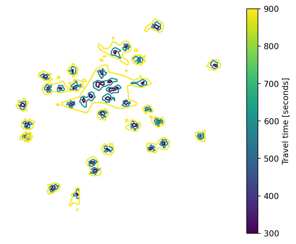
Isochrones of travel time (5, 10 and 15 minutes) around art schools

As you can see above, the isochrones are joined together: we get areas accessible from one or more art schools, not a boundary for each school. It is often easier to work with isochrones as polygons, so let’s build areas from these LineStrings.

1isochrones["polygons"] = shapely.build_area(
    isochrones.geometry 
2).set_crs(isochrones.crs)
3isochrones.set_geometry("polygons").explore('travel_time')

1: Use shapely.build_area to convert linear geometries into areal ones.
2: Set the CRS of the resulting geometries, as Shapely does not pass it through.
3: Set the new polygons as the active geometry and visualise them.

Make this Notebook Trusted to load map: File -> Trust Notebook

Travel-time matrix

The main use case for r5py is computing travel-time matrices. A travel-time matrix contains, as the name suggests, travel times through the network between all pairs of provided origins and destinations. We can illustrate this by computing travel times from all the census areas in our prague dataset to Albertov.

1prague['id'] = prague.index

2origins = prague.set_geometry(prague.centroid)
3destinations = origins.loc[["Albertov"]]

travel_times = r5py.TravelTimeMatrix(
    transport_network,
    origins=origins,
    destinations=destinations,
    departure=datetime.datetime(2026, 10, 22, 10, 30),
4    snap_to_network=True,
)
travel_times

1: Again, each dataset linked to the network needs to have an id column.
2: Snapping to the network requires points rather than polygons.
3: destinations is a single-row GeoDataFrame in this case.
4: We want to snap the locations to the network.

	from_id	to_id	travel_time
0	Běchovice	Albertov	58.0
1	Nová Dubeč	Albertov	58.0
2	Benice	Albertov	71.0
3	Březiněves	Albertov	48.0
4	Dolní Černošice	Albertov	79.0
...	...	...	...
948	K Březiněvsi	Albertov	61.0
949	Ústřední vojenská nemocnice	Albertov	38.0
950	Výzkumný ústav vodohospodářský	Albertov	47.0
951	Sídliště Jalodvorská	Albertov	46.0
952	Strašnice-Za Dráhou	Albertov	49.0

953 rows × 3 columns

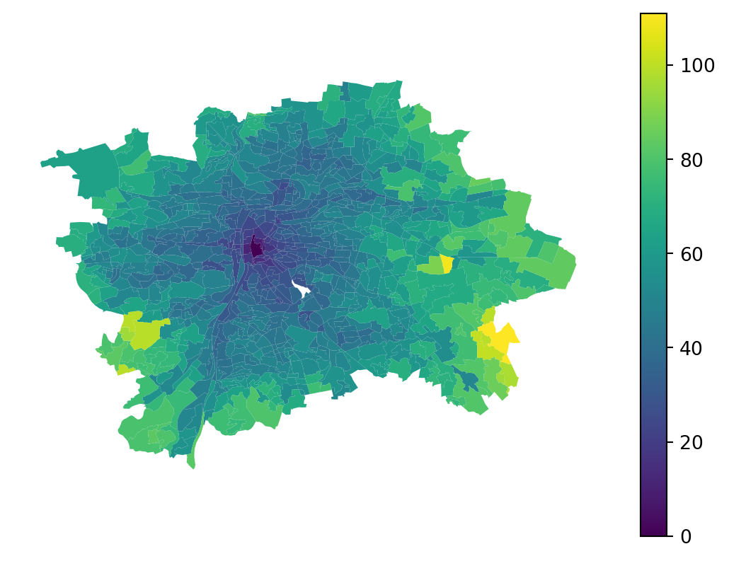
Here, the result shows the time needed to reach Albertov from across the city via public transport.

ax = prague.plot(
1    travel_times.travel_time.values,
    legend=True,
)
ax.set_axis_off()

1: Use .values to pass the underlying numpy.ndarray of values. The Series has a different index from prague, and we want to avoid alignment by index.

Travel time to Albertov using public transport or walking

However, this can be built as a full \(N \times N\) matrix, computing travel times between all pairs of census areas.

travel_times = r5py.TravelTimeMatrix(
    transport_network,
1    origins=origins,
    destinations=origins,
    departure=datetime.datetime(2026, 10, 22, 10, 30),
    snap_to_network=True,
2    max_time=datetime.timedelta(minutes=30),
)
travel_times

1: Both origins and destinations are the same at this point.
2: Set a maximum travel time of 30 minutes, assuming that longer connections are unfeasible.

	from_id	to_id	travel_time
0	Běchovice	Běchovice	0.0
1	Běchovice	Nová Dubeč	15.0
2	Běchovice	Benice	NaN
3	Běchovice	Březiněves	NaN
4	Běchovice	Dolní Černošice	NaN
...	...	...	...
908204	Strašnice-Za Dráhou	K Březiněvsi	NaN
908205	Strašnice-Za Dráhou	Ústřední vojenská nemocnice	NaN
908206	Strašnice-Za Dráhou	Výzkumný ústav vodohospodářský	NaN
908207	Strašnice-Za Dráhou	Sídliště Jalodvorská	NaN
908208	Strašnice-Za Dráhou	Strašnice-Za Dráhou	0.0

908209 rows × 3 columns

Given this is a full \(N*N\) matrix, we can directly convert it to Graph.

transit_graph = graph.Graph.from_adjacency(
1    adjacency=travel_times.dropna(),
    focal_col="from_id",
    neighbor_col="to_id",
    weight_col="travel_time",
)
transit_graph

1: Drop missing values, which represent connections that take longer than 30 minutes (max_time).

<Graph of 953 nodes and 37412 nonzero edges (6 components, 6 isolates) indexed by
 ['Běchovice', 'Nová Dubeč', 'Benice', 'Březiněves', 'Dolní Černošice', ...]>

With this, we already know how to work with the graph.

transit_graph["Albertov"]

neighbor
Betlémský obvod              21.0
Josefov                      26.0
Petrský obvod                29.0
Masarykovo nádraží           26.0
Jindřišský obvod             23.0
                             ... 
V Čelakovského sadech        20.0
U muzea                      22.0
Masarykovo nádraží-východ    28.0
U Fidlovačky-západ           21.0
Obchodní centrum Chodov      29.0
Name: weight, Length: 81, dtype: float64

One issue that remains is that the weight is represented in minutes. We can use the kernels module of libpysal to convert it into a useful weight before generating the Graph.

travel_times["weights"] = kernels.kernel(
    travel_times["travel_time"], 
    bandwidth=30, 
    kernel="bisquare",
    decay=True,
)
travel_times

	from_id	to_id	travel_time	weights
0	Běchovice	Běchovice	0.0	1.0000
1	Běchovice	Nová Dubeč	15.0	0.5625
2	Běchovice	Benice	NaN	NaN
3	Běchovice	Březiněves	NaN	NaN
4	Běchovice	Dolní Černošice	NaN	NaN
...	...	...	...	...
908204	Strašnice-Za Dráhou	K Březiněvsi	NaN	NaN
908205	Strašnice-Za Dráhou	Ústřední vojenská nemocnice	NaN	NaN
908206	Strašnice-Za Dráhou	Výzkumný ústav vodohospodářský	NaN	NaN
908207	Strašnice-Za Dráhou	Sídliště Jalodvorská	NaN	NaN
908208	Strašnice-Za Dráhou	Strašnice-Za Dráhou	0.0	1.0000

908209 rows × 4 columns

The code above converts a travel time of 0 to a weight of 1 and a travel time of 30 to a weight of 0, with a bisquare kernel defining all values in between. You can then use the new column as the weight column when constructing the Graph.

transit_graph_weighted = graph.Graph.from_adjacency(
    adjacency=travel_times.dropna(),
    focal_col="from_id",
    neighbor_col="to_id",
    weight_col="weights",
)

You can see that the weights are now as expected for spatial modelling tasks.

transit_graph_weighted["Albertov"]

neighbor
Betlémský obvod              0.260100
Josefov                      0.061946
Petrský obvod                0.004298
Masarykovo nádraží           0.061946
Jindřišský obvod             0.169927
                               ...   
V Čelakovského sadech        0.308642
U muzea                      0.213649
Masarykovo nádraží-východ    0.016612
U Fidlovačky-západ           0.260100
Obchodní centrum Chodov      0.004298
Name: weight, Length: 81, dtype: float64

This can be nicely illustrated on a map. Notice the discontinuity caused by the locations of public transit stops.

ax = prague.assign(weight=transit_graph_weighted["Albertov"]).plot(
    'weight', legend=True, tiles=True, alpha=.7,
)
ax.set_axis_off()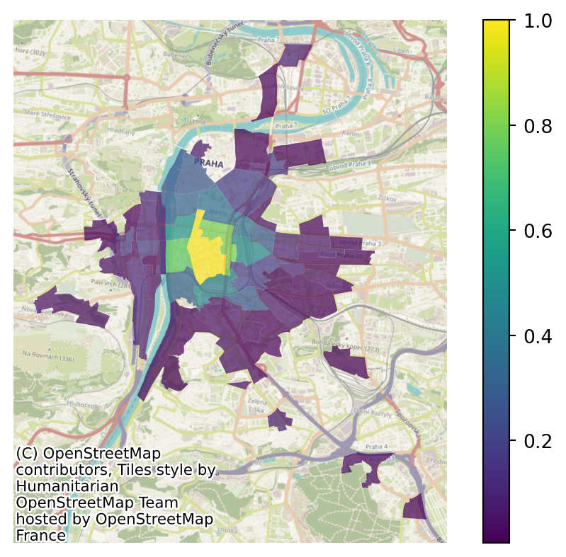

Spatial interaction weight derived from public transport

See the effects of the spatial graph defined in this way on the spatial lag of population.

lagged_population = transit_graph_weighted.lag(prague["n_people"])

prague.explore(lagged_population)

Make this Notebook Trusted to load map: File -> Trust Notebook

The main public transport routes are noticeable in the result.

Additional reading

For more resources on using r5py, you can check the documentation or the tutorial written by Henrikki Tenkanen, Christoph Fink and Willem Klumpenhouwer.

A general (lower-level) overview of spatial networks is available in the Introduction to Spatial Networks using Python by Michael Dorman.