Clustering and regionalisation

This session is all about finding groups of similar observations in data using clustering techniques.

Many questions and topics are complex phenomena that involve several dimensions and are hard to summarise into a single variable. In statistical terms, you call this family of problems multivariate, as opposed to univariate cases where only a single variable is considered in the analysis. Clustering tackles this kind of questions by reducing their dimensionality -the number of relevant variables the analyst needs to look at - and converting it into a more intuitive set of classes that even non-technical audiences can look at and make sense of. For this reason, it is widely used in applied contexts such as policymaking or marketing. In addition, since these methods do not require many preliminary assumptions about the structure of the data, it is a commonly used exploratory tool, as it can quickly give clues about the shape, form and content of a dataset.

The basic idea of statistical clustering is to summarise the information contained in several variables by creating a relatively small number of categories. Each observation in the dataset is then assigned to one, and only one, category depending on its values for the variables originally considered in the classification. If done correctly, the exercise reduces the complexity of a multi-dimensional problem while retaining all the meaningful information contained in the original dataset. This is because once classified, the analyst only needs to look at in which category every observation falls into, instead of considering the multiple values associated with each of the variables and trying to figure out how to put them together in a coherent sense. When the clustering is performed on observations that represent areas, the technique is often called geodemographic analysis.

Although there exist many techniques to statistically group observations in a dataset, all of them are based on the premise of using a set of attributes to define classes or categories of observations that are similar within each of them, but differ between groups. How similarity within groups and dissimilarity between them is defined and how the classification algorithm is operationalised is what makes techniques differ and also what makes each of them particularly well suited for specific problems or types of data.

In the case of analysing spatial data, there is a subset of methods that are of particular interest for many common cases in Spatial Data Science. These are the so-called regionalisation techniques. Regionalisation methods can also take many forms and faces but, at their core, they all involve statistical clustering of observations with the additional constraint that observations need to be geographical neighbours to be in the same category. Because of this, rather than category, you will use the term area for each observation and region for each category, hence regionalisation, the construction of regions from smaller areas.

The Python package you will use for clustering today is called scikit-learn and can be imported as sklearn.

import geopandas as gpd
import pandas as pd
import seaborn as sns
from libpysal import graph
from sklearn import cluster

Attribute-based clustering

In this session, you will be working with another dataset you should already be familiar with - the Scottish Index of Multiple Deprivation. This time, you will focus only on the area of Edinburgh prepared for this course.

Scottish Index of Multiple Deprivation

As always, the table can be read from the site:

simd = gpd.read_file(
    "https://martinfleischmann.net/sds/clustering/data/edinburgh_simd_2020.gpkg"
)

Alternative

Instead of reading the file directly off the web, it is possible to download it manually, store it on your computer, and read it locally. To do that, you can follow these steps:

Download the file by right-clicking on this link and saving the file
Place the file in the same folder as the notebook where you intend to read it
Replace the code in the cell above with:

simd = gpd.read_file(
    "edinburgh_simd_2020.gpkg",
)

Inspect the structure of the table:

simd.info()

<class 'geopandas.geodataframe.GeoDataFrame'>
RangeIndex: 597 entries, 0 to 596
Data columns (total 52 columns):
 #   Column      Non-Null Count  Dtype   
---  ------      --------------  -----   
 0   DataZone    597 non-null    object  
 1   DZName      597 non-null    object  
 2   LAName      597 non-null    object  
 3   SAPE2017    597 non-null    int64   
 4   WAPE2017    597 non-null    int64   
 5   Rankv2      597 non-null    int64   
 6   Quintilev2  597 non-null    int64   
 7   Decilev2    597 non-null    int64   
 8   Vigintilv2  597 non-null    int64   
 9   Percentv2   597 non-null    int64   
 10  IncRate     597 non-null    object  
 11  IncNumDep   597 non-null    int64   
 12  IncRankv2   597 non-null    float64 
 13  EmpRate     597 non-null    object  
 14  EmpNumDep   597 non-null    int64   
 15  EmpRank     597 non-null    float64 
 16  HlthCIF     597 non-null    int64   
 17  HlthAlcSR   597 non-null    int64   
 18  HlthDrugSR  597 non-null    int64   
 19  HlthSMR     597 non-null    int64   
 20  HlthDprsPc  597 non-null    object  
 21  HlthLBWTPc  597 non-null    object  
 22  HlthEmergS  597 non-null    int64   
 23  HlthRank    597 non-null    int64   
 24  EduAttend   597 non-null    object  
 25  EduAttain   597 non-null    float64 
 26  EduNoQuals  597 non-null    int64   
 27  EduPartici  597 non-null    object  
 28  EduUniver   597 non-null    object  
 29  EduRank     597 non-null    int64   
 30  GAccPetrol  597 non-null    float64 
 31  GAccDTGP    597 non-null    float64 
 32  GAccDTPost  597 non-null    float64 
 33  GAccDTPsch  597 non-null    float64 
 34  GAccDTSsch  597 non-null    float64 
 35  GAccDTRet   597 non-null    float64 
 36  GAccPTGP    597 non-null    float64 
 37  GAccPTPost  597 non-null    float64 
 38  GAccPTRet   597 non-null    float64 
 39  GAccBrdbnd  597 non-null    object  
 40  GAccRank    597 non-null    int64   
 41  CrimeCount  597 non-null    int64   
 42  CrimeRate   597 non-null    int64   
 43  CrimeRank   597 non-null    float64 
 44  HouseNumOC  597 non-null    int64   
 45  HouseNumNC  597 non-null    int64   
 46  HouseOCrat  597 non-null    object  
 47  HouseNCrat  597 non-null    object  
 48  HouseRank   597 non-null    float64 
 49  Shape_Leng  597 non-null    float64 
 50  Shape_Area  597 non-null    float64 
 51  geometry    597 non-null    geometry
dtypes: float64(16), geometry(1), int64(22), object(13)
memory usage: 242.7+ KB

Before you jump into exploring the data, one additional step that will come in handy down the line. Not every variable in the table is an attribute that you will want for the clustering. In particular, you are interested in sub-ranks based on individual SIMD domains, so you will only consider those. Hence, first manually write them so they are easier to subset:

subranks = [
    "IncRankv2",
    "EmpRank",
    "HlthRank",
    "EduRank",
    "GAccRank",
    "CrimeRank",
    "HouseRank"
]

You can quickly familiarise yourself with those variables by plotting a few maps like the one below to build your intuition about what is going to happen.

simd[["IncRankv2", "geometry"]].explore("IncRankv2", tiles="CartoDB Positron", tooltip=False)

Make this Notebook Trusted to load map: File -> Trust Notebook

You can see a decent degree of spatial variation between different sub-ranks. Even though you only have seven variables, it is very hard to “mentally overlay” all of them to come up with an overall assessment of the nature of each part of Edinburgh. For bivariate correlations, a useful tool is the correlation matrix plot, available in seaborn:

_ = sns.pairplot(simd[subranks],height=1, plot_kws={"s":1})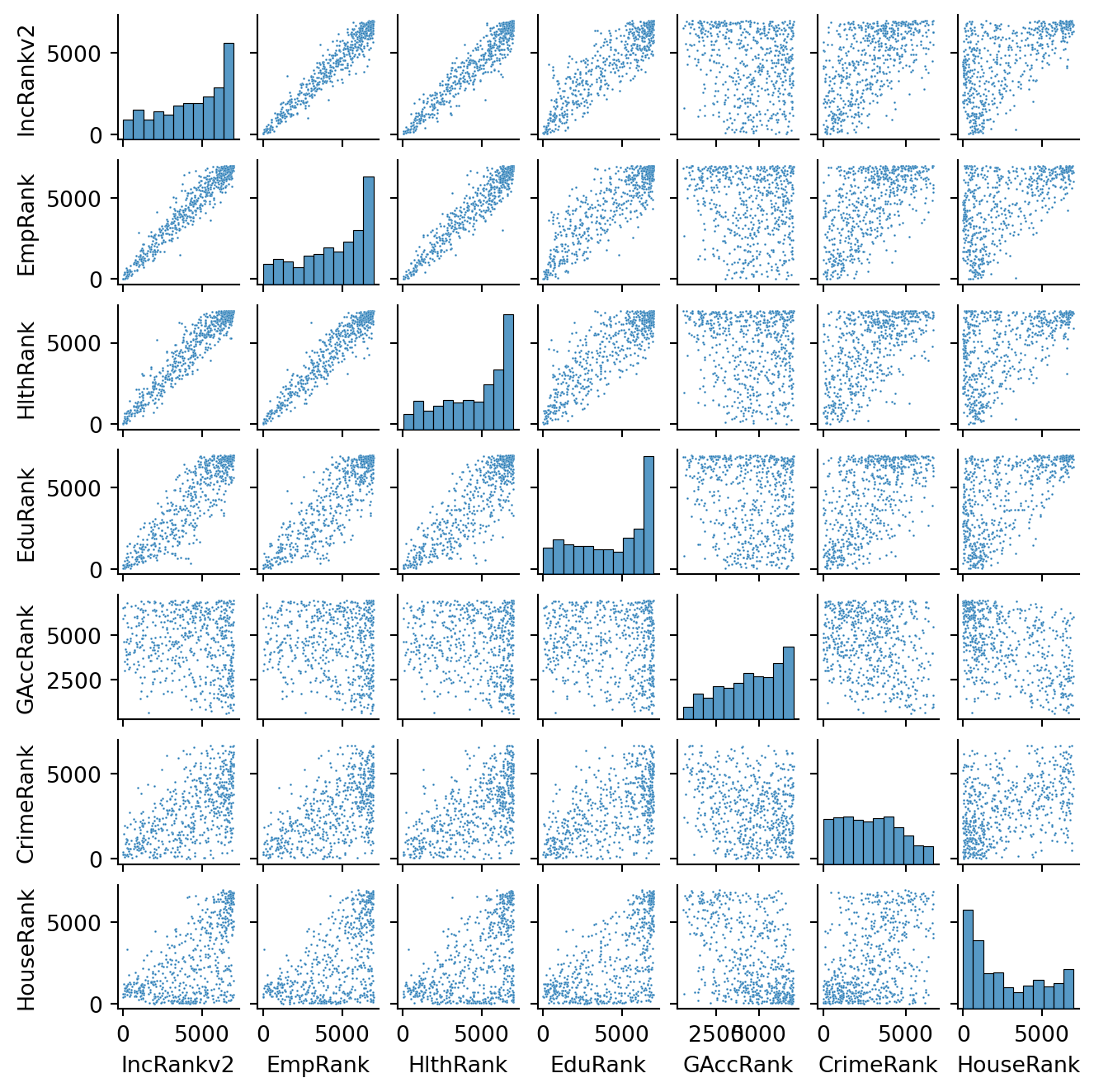

This is helpful to consider uni and bivariate questions such as: what is the relationship between the ranks? Is health correlated with income? However, sometimes, this is not enough and you are interested in more sophisticated questions that are truly multivariate and, in these cases, the figure above cannot help us. For example, it is not straightforward to answer questions like: what are the main characteristics of the South of Edinburgh? What areas are similar to the core of the city? Are the East and West of Edinburgh similar in terms of deprivation levels? For these kinds of multi-dimensional questions -involving multiple variables at the same time- you require a truly multidimensional method like statistical clustering.

K-Means

A cluster analysis involves the classification of the areas that make up a geographical map into groups or categories of observations that are similar within each other but different between them. The classification is carried out using a statistical clustering algorithm that takes as input a set of attributes and returns the group (“labels” in the terminology) each observation belongs to. Depending on the particular algorithm employed, additional parameters, such as the desired number of clusters employed or more advanced tuning parameters (e.g. bandwith, radius, etc.), also need to be entered as inputs. For your classification of SIMD in Edinburgh, you will start with one of the most popular clustering algorithms: K-means. This technique only requires as input the observation attributes and the final number of groups that you want it to cluster the observations into. In your case, you will use five to begin with as this will allow us to have a closer look into each of them.

Although the underlying algorithm is not trivial, running K-means in Python is streamlined thanks to scikit-learn. Similar to the extensive set of available algorithms in the library, its computation is a matter of two lines of code. First, you need to specify the parameters in the KMeans method (which is part of scikit-learn’s cluster submodule). Note that, at this point, you do not even need to pass the data:

1kmeans5 = cluster.KMeans(n_clusters=5, random_state=42)

1: n_clusters specifies the number of clusters you want to get and random_state sets the random generator to a known state, ensuring that the result is always the same.

This sets up an object that holds all the parameters required to run the algorithm. To actually run the algorithm on the attributes, you need to call the fit method in kmeans5:

1kmeans5.fit(simd[subranks])

1: fit() takes an array of data; therefore, pass the columns of simd with sub-ranks and run the clustering algorithm on that.

KMeans(n_clusters=5, random_state=42)

In a Jupyter environment, please rerun this cell to show the HTML representation or trust the notebook.
On GitHub, the HTML representation is unable to render, please try loading this page with nbviewer.org.

The kmeans5 object now contains several components that can be useful for an analysis. For now, you will use the labels, which represent the different categories in which you have grouped the data. Remember, in Python, life starts at zero, so the group labels go from zero to four. Labels can be extracted as follows:

kmeans5.labels_

array([2, 2, 2, 2, 3, 2, 2, 2, 2, 3, 2, 3, 4, 4, 2, 2, 2, 2, 2, 2, 2, 2,
       2, 2, 2, 2, 2, 2, 2, 2, 2, 2, 1, 1, 1, 1, 3, 1, 1, 1, 1, 3, 1, 1,
       1, 1, 1, 3, 3, 3, 3, 3, 3, 1, 1, 1, 1, 1, 1, 1, 1, 1, 1, 1, 3, 1,
       1, 3, 0, 3, 0, 3, 3, 3, 3, 3, 1, 1, 3, 3, 0, 3, 3, 1, 0, 0, 0, 0,
       4, 0, 0, 2, 2, 2, 2, 2, 2, 2, 2, 0, 0, 4, 2, 2, 2, 2, 2, 1, 1, 3,
       3, 3, 3, 1, 1, 3, 3, 2, 2, 2, 2, 2, 2, 2, 2, 2, 2, 2, 2, 2, 2, 2,
       3, 2, 3, 2, 3, 1, 1, 1, 1, 1, 3, 1, 3, 1, 1, 3, 1, 1, 1, 3, 1, 1,
       1, 3, 4, 2, 2, 4, 4, 4, 2, 3, 1, 1, 1, 3, 1, 1, 2, 2, 2, 2, 2, 3,
       2, 4, 1, 3, 2, 0, 0, 0, 0, 0, 0, 0, 0, 2, 4, 4, 2, 0, 0, 0, 0, 0,
       0, 0, 0, 0, 0, 0, 0, 0, 0, 4, 2, 4, 4, 0, 0, 0, 0, 3, 4, 0, 4, 0,
       0, 0, 0, 0, 0, 0, 0, 0, 0, 0, 0, 3, 0, 3, 3, 1, 3, 3, 3, 1, 3, 3,
       3, 0, 3, 3, 3, 3, 3, 0, 0, 0, 0, 0, 0, 0, 3, 3, 3, 3, 3, 3, 1, 3,
       3, 3, 3, 1, 3, 1, 3, 3, 3, 0, 3, 3, 4, 0, 0, 2, 2, 4, 1, 2, 1, 3,
       1, 1, 1, 1, 1, 1, 1, 1, 1, 1, 1, 1, 1, 1, 3, 3, 3, 3, 2, 2, 2, 4,
       4, 4, 4, 3, 4, 3, 3, 1, 3, 3, 4, 4, 4, 4, 3, 4, 4, 3, 1, 3, 0, 1,
       4, 4, 4, 4, 3, 1, 1, 3, 1, 1, 1, 1, 1, 1, 3, 0, 0, 3, 3, 4, 3, 1,
       3, 0, 3, 3, 3, 1, 3, 1, 1, 3, 0, 3, 1, 3, 0, 3, 1, 3, 1, 3, 1, 1,
       3, 3, 1, 1, 3, 3, 3, 3, 3, 3, 3, 3, 1, 3, 0, 3, 3, 3, 0, 0, 0, 0,
       1, 3, 3, 3, 3, 0, 0, 1, 0, 4, 4, 4, 4, 3, 4, 0, 4, 4, 4, 2, 4, 4,
       4, 3, 0, 0, 0, 0, 0, 0, 0, 0, 0, 3, 0, 0, 0, 0, 3, 4, 0, 0, 0, 0,
       0, 4, 0, 0, 4, 0, 4, 2, 4, 0, 4, 0, 0, 0, 0, 0, 4, 4, 0, 4, 4, 3,
       4, 4, 2, 4, 2, 2, 4, 2, 2, 2, 0, 2, 2, 4, 4, 2, 4, 2, 4, 4, 1, 1,
       3, 1, 1, 1, 1, 1, 1, 1, 3, 3, 3, 2, 3, 3, 4, 1, 1, 1, 1, 3, 1, 1,
       1, 1, 1, 3, 3, 1, 1, 1, 1, 3, 1, 1, 4, 4, 0, 2, 4, 4, 2, 2, 2, 2,
       2, 2, 2, 4, 3, 3, 1, 1, 1, 3, 2, 2, 3, 1, 3, 2, 2, 2, 2, 4, 4, 2,
       4, 2, 2, 4, 2, 2, 4, 4, 3, 4, 4, 0, 3, 3, 4, 3, 3, 3, 3, 4, 4, 3,
       0, 0, 2, 3, 2, 3, 2, 3, 2, 1, 3, 2, 2, 2, 4, 2, 4, 3, 3, 4, 1, 4,
       2, 2, 2], dtype=int32)

Each number represents a different category, so two observations with the same number belong to the same group. The labels are returned in the same order as the input attributes were passed in, which means you can append them to the original table of data as an additional column:

simd["kmeans_5"] = kmeans5.labels_
simd["kmeans_5"].head()

0    2
1    2
2    2
3    2
4    3
Name: kmeans_5, dtype: int32

It is useful to display the categories created on a map to better understand the classification you have just performed. For this, you will use a unique values choropleth, which will automatically assign a different colour to each category:

simd[["kmeans_5", 'geometry']].explore("kmeans_5", categorical=True, tiles="CartoDB Positron")

Make this Notebook Trusted to load map: File -> Trust Notebook

The map above represents the geographical distribution of the five categories created by the K-means algorithm. A quick glance shows a strong spatial structure in the distribution of the colours: group 3 (grey) is mostly in central areas and towards the west, group 1 (green) covers peripheries and so on, but not all clusters are equally represented.

Not all data can go to clustering in their raw form

Clustering, as well as many other statistical methods, often depends on pairwise distances between observations based on the variables passed. That has, in practice, serious implications on what can be used. For example, you cannot use one variable that is limited to a range between 0 and 1 and another that stretches from 0 to 100 000. The latter would dominate the distance and the former would have negligible effect on the results. For these reasons, the data usually need to be standardised in some way. See the Data section of the chapter Clustering and Regionalization from the Geographic Data Science with Python by Rey, Arribas-Bel, and Wolf (2023) for more details.

In this case, all the sub-ranks are defined the same way so you don’t need any standardisation.

Exploring the nature of the categories

Once you have a sense of where and how the categories are distributed over space, it is also useful to explore them statistically. This will allow you to characterise them, giving you an idea of the kind of observations subsumed into each of them. As a first step, find how many observations are in each category. To do that, you will make use of the groupby operator introduced before, combined with the function size, which returns the number of elements in a subgroup:

k5sizes = simd.groupby('kmeans_5').size()
k5sizes

kmeans_5
0    110
1    129
2    119
3    154
4     85
dtype: int64

The groupby operator groups a table (DataFrame) using the values in the column provided (kmeans_5) and passes them onto the function provided aftwerards, which in this case is size. Effectively, what this does is to groupby the observations by the categories created and count how many of them each contains. For a more visual representation of the output, a bar plot is a good alternative:

_ = k5sizes.plot.bar()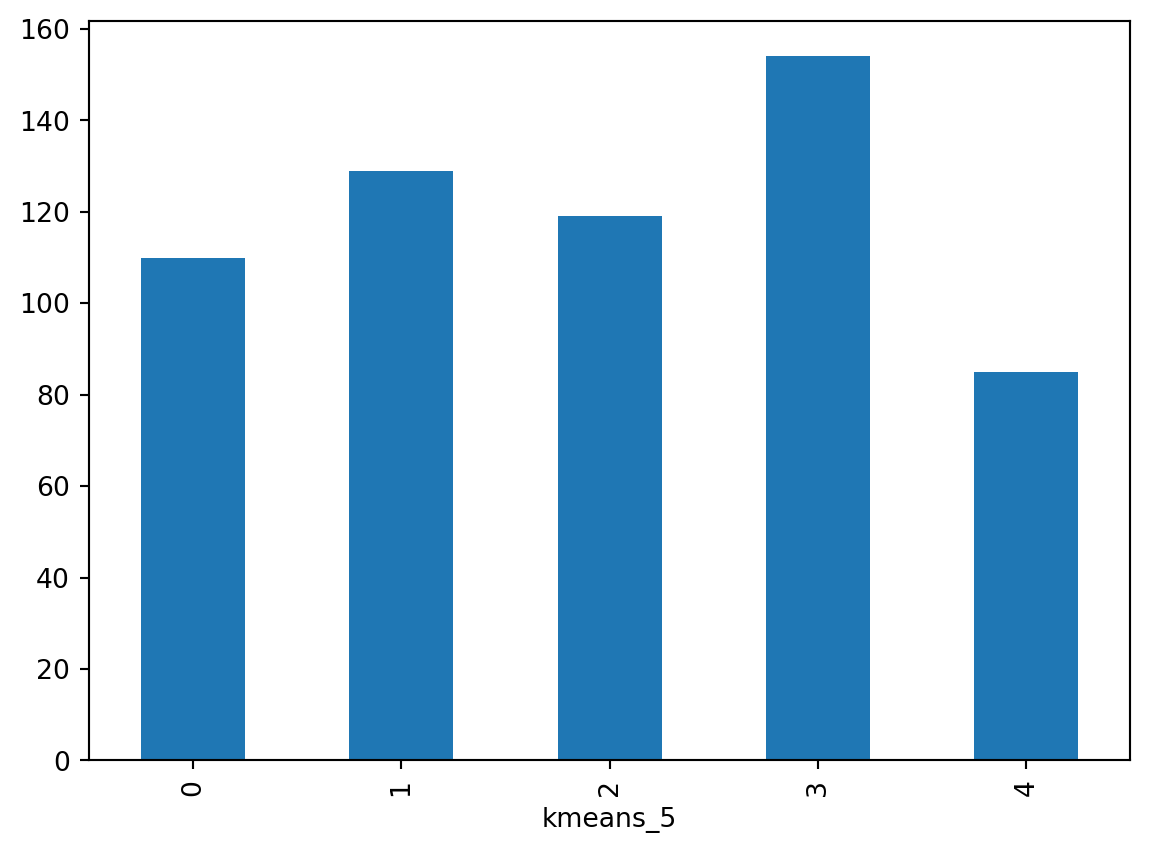

As you suspected from the map, groups vary in size, with group 2 having over 200 observations, groups 0, 1 and 4 over 100 and a group 3 having 74 observations.

In order to describe the nature of each category, you can look at the values of each of the attributes you have used to create them in the first place. Remember you used the sub-ranks on many aspects of deprivation to create the classification, so you can begin by checking the average value of each. To do that in Python, you will rely on the groupby operator which you will combine with the function mean:

1k5_means = simd.groupby('kmeans_5')[subranks].mean()
2k5_means.T

1: Use groupby to calculate mean per each sub-rank.
2: Transpose the table so it is not too wide

kmeans_5	0	1	2	3	4
IncRankv2	5788.150000	1294.806202	6223.117647	3618.136364	5979.135294
EmpRank	6096.622727	1380.275194	6216.075630	3809.990260	6033.841176
HlthRank	6265.381818	1467.255814	6235.848739	3936.883117	6022.294118
EduRank	5780.872727	1253.434109	6314.697479	3125.474026	6241.117647
GAccRank	5614.745455	4670.139535	2221.134454	5015.285714	5148.000000
CrimeRank	3639.209091	1250.546512	4363.285714	2322.129870	3366.088235
HouseRank	1247.836364	1024.294574	5677.218487	1469.396104	5096.364706

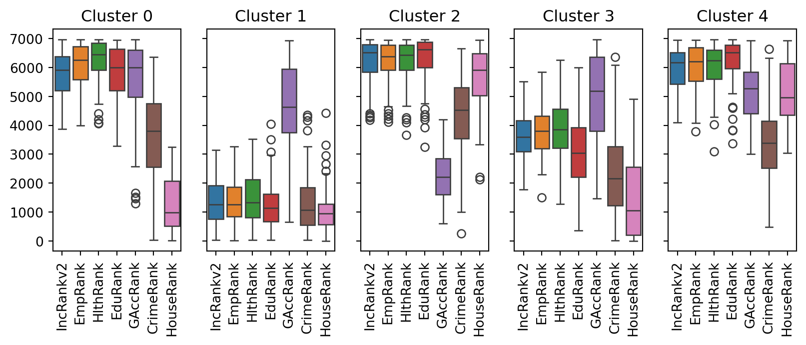
When interpreting the values, remember that a lower value represents higher deprivation. While the results seem plausible and there are ways of interpreting them, you haven’t used any spatial methods.

Selecting the optimal number of clusters

K-means (and a lot of other algorithms) requires a number of clusters as an input argument. But how do you know what is the right number? A priori, you usually dont. That is why the clustering tasks normally contains a step aiming at determining the optimal number of classes. The most common method is a so-called “elbow method”.

The main prinicple is simple. You do clustering for a range of options, typically from 2 to \(n\). Here, you can test all the options between 2 and 15, for example. For each result, you measure some metric of cluster fit. The simple elbow method is using inertia, which is a sum of squared distances of samples to their closest cluster center. But you can also use other metrics like Silhouette score or Calinski-Harabasz score.

Loop over the options and save inertias per each option.

1inertias = {}

2for k in range(2, 15):
3    kmeans = cluster.KMeans(n_clusters=k, random_state=42)
    kmeans.fit(simd[subranks])
4    inertias[k] = kmeans.inertia_

1: Create an empty dictionary to hold the results computed in the loop.
2: Loop over a range of values from two to fifteen.
3: Generate clustering result for each k.
4: Save the inertia value to the dictionary.

Now you can create the elbow plot. On the resulting curve, you shall be looking for an “elbow”, a point where the inertia stops decreasing “fast enough”, i.e. where the additional cluster does not bring much to the model. In this case, it would be eithher 4 or 6.

_ = pd.Series(inertias).plot()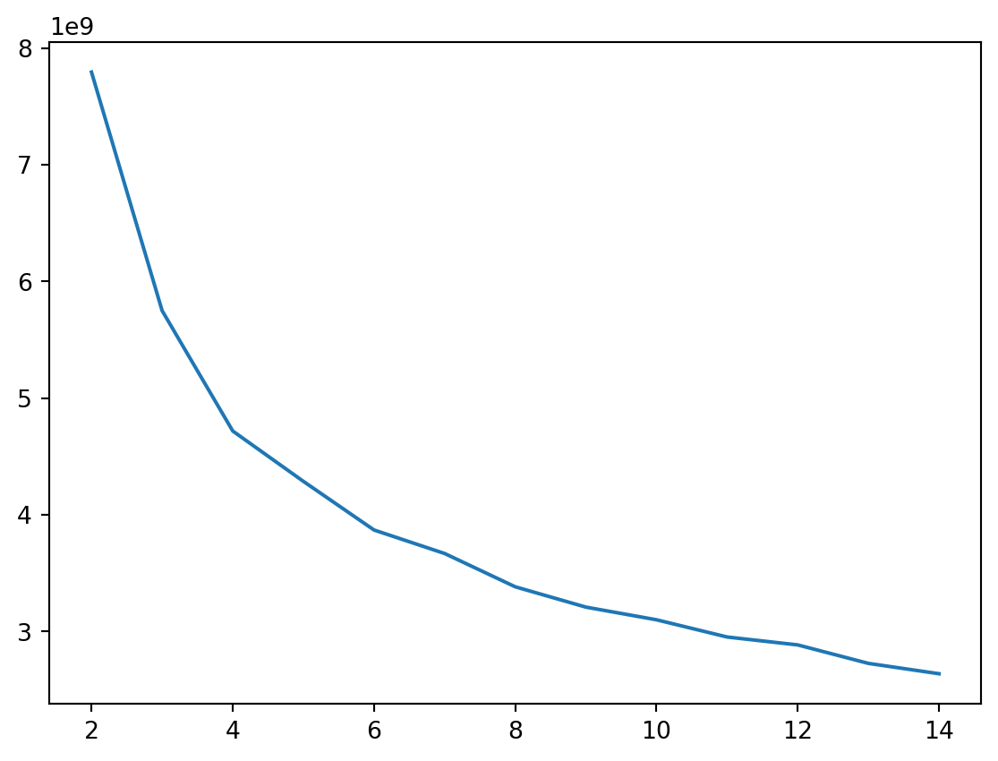

Check the ‘optimal’ result

Now that you know the optimal number, check how it looks on the map and what is the main difference between 5, picked randomly, and the value derived from the elbow plot.

The issue with the elbow plot is that the detection of the optimal number tends to be ambiguous but thanks to its simplicity, it is used anyway. However, there is a range of other methods that may provide a better understanding of cluster behaviour, like a clustergram or a silhouette analysis, both of which are out of scope of this material.

Spatially-lagged clustering

K-means (in its standard implementation) does not have a way of including of spatial restriction. However, it is still a very powerful and efficient algorithm and it would be a shame not to make a use of it when dealing with spatial data. To include spatial dimension in (nearly any) non-spatial model, you can use spatially lagged variables. Instead of passing in only the variables observed in each data zone, you also pass in their spatial lags. Due to the nature of the spatial lag, this encodes a certain degree of spatial contiguity into data that are being clustered, often resulting in spatially more homogenous areas.

Start with building a queen contiguity weights matrix.

queen = graph.Graph.build_contiguity(simd)

As always, you will need a row-standardised matrix.

queen_row = queen.transform("R")

You need a lagged version of each of the sub-ranks as its own, new column. You can loop through the subranks list and create them one by one, using a basic for loop.

1for column in subranks:
2    simd[column + "_lag"] = queen_row.lag(simd[column])

1: For loop picks an item form subranks, assigns it to a column variable and runs the code inside the loop. Then it picks the second item from the list and runs the code again, with the second item as column. And so on until it covers the whole iterable item.
2: In the first pass, column contains "IncRankv2", so create a column called "IncRankv2_lag" with a spatial lag.

You can check that the simd table now has new columns.

simd.info()

<class 'geopandas.geodataframe.GeoDataFrame'>
RangeIndex: 597 entries, 0 to 596
Data columns (total 60 columns):
 #   Column         Non-Null Count  Dtype   
---  ------         --------------  -----   
 0   DataZone       597 non-null    object  
 1   DZName         597 non-null    object  
 2   LAName         597 non-null    object  
 3   SAPE2017       597 non-null    int64   
 4   WAPE2017       597 non-null    int64   
 5   Rankv2         597 non-null    int64   
 6   Quintilev2     597 non-null    int64   
 7   Decilev2       597 non-null    int64   
 8   Vigintilv2     597 non-null    int64   
 9   Percentv2      597 non-null    int64   
 10  IncRate        597 non-null    object  
 11  IncNumDep      597 non-null    int64   
 12  IncRankv2      597 non-null    float64 
 13  EmpRate        597 non-null    object  
 14  EmpNumDep      597 non-null    int64   
 15  EmpRank        597 non-null    float64 
 16  HlthCIF        597 non-null    int64   
 17  HlthAlcSR      597 non-null    int64   
 18  HlthDrugSR     597 non-null    int64   
 19  HlthSMR        597 non-null    int64   
 20  HlthDprsPc     597 non-null    object  
 21  HlthLBWTPc     597 non-null    object  
 22  HlthEmergS     597 non-null    int64   
 23  HlthRank       597 non-null    int64   
 24  EduAttend      597 non-null    object  
 25  EduAttain      597 non-null    float64 
 26  EduNoQuals     597 non-null    int64   
 27  EduPartici     597 non-null    object  
 28  EduUniver      597 non-null    object  
 29  EduRank        597 non-null    int64   
 30  GAccPetrol     597 non-null    float64 
 31  GAccDTGP       597 non-null    float64 
 32  GAccDTPost     597 non-null    float64 
 33  GAccDTPsch     597 non-null    float64 
 34  GAccDTSsch     597 non-null    float64 
 35  GAccDTRet      597 non-null    float64 
 36  GAccPTGP       597 non-null    float64 
 37  GAccPTPost     597 non-null    float64 
 38  GAccPTRet      597 non-null    float64 
 39  GAccBrdbnd     597 non-null    object  
 40  GAccRank       597 non-null    int64   
 41  CrimeCount     597 non-null    int64   
 42  CrimeRate      597 non-null    int64   
 43  CrimeRank      597 non-null    float64 
 44  HouseNumOC     597 non-null    int64   
 45  HouseNumNC     597 non-null    int64   
 46  HouseOCrat     597 non-null    object  
 47  HouseNCrat     597 non-null    object  
 48  HouseRank      597 non-null    float64 
 49  Shape_Leng     597 non-null    float64 
 50  Shape_Area     597 non-null    float64 
 51  geometry       597 non-null    geometry
 52  kmeans_5       597 non-null    int32   
 53  IncRankv2_lag  597 non-null    float64 
 54  EmpRank_lag    597 non-null    float64 
 55  HlthRank_lag   597 non-null    float64 
 56  EduRank_lag    597 non-null    float64 
 57  GAccRank_lag   597 non-null    float64 
 58  CrimeRank_lag  597 non-null    float64 
 59  HouseRank_lag  597 non-null    float64 
dtypes: float64(23), geometry(1), int32(1), int64(22), object(13)
memory usage: 277.6+ KB

Let’s create a list of these new columns.

1subranks_lag = [column + "_lag" for column in subranks]
subranks_lag

1: This is also a for loop but in the form of a list comprehension. The whole loop is there to fill the values of the list.

['IncRankv2_lag',
 'EmpRank_lag',
 'HlthRank_lag',
 'EduRank_lag',
 'GAccRank_lag',
 'CrimeRank_lag',
 'HouseRank_lag']

Now, combine the list of original variables and those with a lag to make it easier to pass the data to K-means.

1subranks_spatial = subranks + subranks_lag
subranks_spatial

1: With arrays like pandas.Series, this would perform element-wise addition. With lists, this combines them together.

['IncRankv2',
 'EmpRank',
 'HlthRank',
 'EduRank',
 'GAccRank',
 'CrimeRank',
 'HouseRank',
 'IncRankv2_lag',
 'EmpRank_lag',
 'HlthRank_lag',
 'EduRank_lag',
 'GAccRank_lag',
 'CrimeRank_lag',
 'HouseRank_lag']

Initialise a new clustering model. Again, you could use the elbow or other methods to determine the optimal number. Note that it may be different than before.

kmeans5_lag = cluster.KMeans(n_clusters=5, random_state=42)

And run it using the new subset, adding lagged variables on top of the original ones.

kmeans5_lag.fit(simd[subranks_spatial])

KMeans(n_clusters=5, random_state=42)

Assing the result as a column.

simd["kmeans_5_lagged"] = kmeans5_lag.labels_

And explore as a map.

simd[["kmeans_5_lagged", 'geometry']].explore("kmeans_5_lagged", categorical=True, tiles="CartoDB Positron")

Make this Notebook Trusted to load map: File -> Trust Notebook

Comparing the spatially-lagged clusters with the original results shows that the new clusters are much more homogenous spatially, delineating relatively compact regions of data zones.

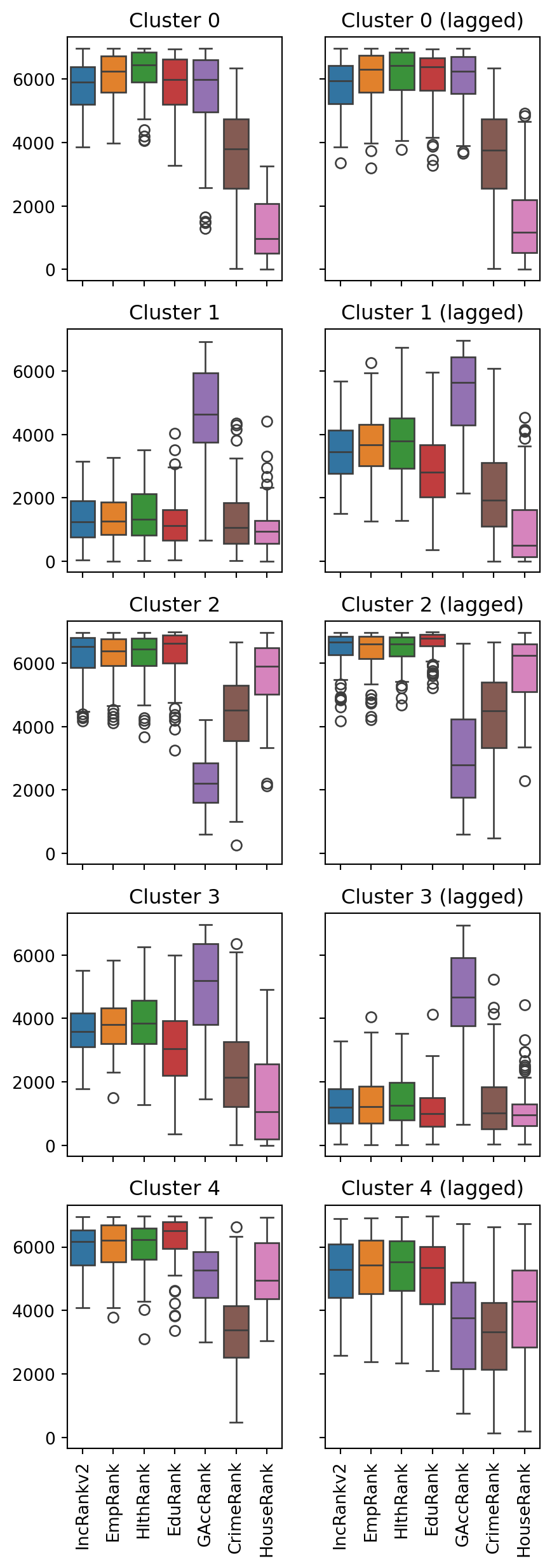
As you have seen, the essence of this approach is to group areas based on a purely statistical basis: where each area is located is irrelevant for the label it receives from the clustering algorithm. In many contexts, this is not only permissible but even desirable, as the interest is to see if particular combinations of values are distributed over space in any discernible way. However, in other contexts, you may be interested in creating groups of observations that follow certain spatial constraints. For that, you now turn to regionalisation techniques.

Spatially-constrained clustering (regionalisation)

Regionalisation is the subset of clustering techniques that impose a spatial constraint on the classification. In other words, the result of a regionalisation algorithm contains areas that are spatially contiguous. While spatially lagged clustering may result in contiguous areas, it does not enforce them. Regionalisation does. Effectively, what this means is that these techniques aggregate areas into a smaller set of larger ones, called regions. In this context, then, areas are nested within regions. Real-world examples of this phenomenon include counties within states or, in Scotland, data zones (DZName) into Local Authorities (LAName). The difference between those examples and the output of a regionalisation algorithm is that while the former are aggregated based on administrative principles, the latter follows a statistical technique that, very much the same as in the standard statistical clustering, groups together areas that are similar on the basis of a set of attributes. Only now, such statistical clustering is spatially constrained.

As in the non-spatial case, there are many different algorithms to perform regionalization, and they all differ on details relating to the way they measure (dis)similarity, the process to regionalize, etc. However, same as above too, they all share a few common aspects. In particular, they all take a set of input attributes and a representation of space in the form of a binary spatial weights matrix. Depending on the algorithm, they also require the desired number of output regions into which the areas are aggregated.

To illustrate these concepts, you will run a regionalisation algorithm on the SIMD data you have been using. In this case, the goal will be to delineate regions of similar levels of deprivation. In this way, the resulting regions will represent a consistent set of areas that are similar to each other in terms of the SIMD sub-ranks received.

At this point, you have all the pieces needed to run a regionalisation algorithm since you have already created a queen contiguity matrix above. For this example, you will use a spatially-constrained version of the agglomerative algorithm. This is a similar approach to that used above (the inner workings of the algorithm are different, however) with the difference that, in this case, observations can only be labelled in the same group if they are spatial neighbours, as defined by your spatial weights matrix queen. The way to interact with the algorithm is very similar to that above. You first set the parameters:

1agg5 = cluster.AgglomerativeClustering(n_clusters=5, connectivity=queen.sparse)

1: scikit-learn expects the connectivity graph as a sparse array, rather than a libpysal.Graph.

And you can run the algorithm by calling fit:

agg5.fit(simd[subranks])

AgglomerativeClustering(connectivity=<Compressed Sparse Row sparse array of dtype 'float64'
    with 3436 stored elements and shape (597, 597)>,
                        n_clusters=5)

And then you append the labels to the table in the same way as before:

simd["agg_5"] = agg5.labels_

At this point, the column agg_5 is no different than kmeans_5: a categorical variable that can be mapped into a unique values choropleth. In fact, the following code snippet is exactly the same as before, only replacing the name of the variable to be mapped and the title:

simd[["agg_5", 'geometry']].explore("agg_5", categorical=True, tiles="CartoDB Positron")

Make this Notebook Trusted to load map: File -> Trust Notebook

Optimal number of clusters

Five might not be the optimal number of classes when we deal with regionalisation as two regions of the same characteristics may have to be disconnected. Therefore, the number of clusters will typically be a bit higher than in the non-spatial case. Test yourself what should be the optimal number here. Note that AgglomerativeClustering does not contain inertia_ property so you will need to derive some metric yourself.

Extracting the region boundaries

With this result, you may want to extract the boundaries of the regions, rather than labels of individual data zones. To create the new boundaries “properly”, you need to dissolve all the polygons in each category into a single one. This is a standard GIS operation that is supported by geopandas.

1simd_regions = simd[["agg_5", "geometry"]].dissolve("agg_5")
simd_regions

1: If you are interested only in the boundaries, you can select just the two relevant colunms and dissolve geoemtries by values in the "agg_5" column. This uses groubpy under the hood, so you can potentially also aggregate other variables. See the documentation on how.

	geometry
agg_5
0	MULTIPOLYGON (((318678.9 664014.8, 318639 6639...
1	POLYGON ((324481 670725, 324468.497 670710.774...
2	POLYGON ((328123.999 667900.999, 328116 667864...
3	POLYGON ((322398.424 674897.483, 322366.127 67...
4	POLYGON ((320641 669158, 320555 669108, 320539...

simd_regions.reset_index().explore("agg_5", categorical=True, tiles="CartoDB Positron")

Make this Notebook Trusted to load map: File -> Trust Notebook

Additional reading

Have a look at the chapter Clustering and Regionalization from the Geographic Data Science with Python by Rey, Arribas-Bel, and Wolf (2023) for more details and some other extensions.

Acknowledgements

This section is derived from A Course on Geographic Data Science by Arribas-Bel (2019), licensed under CC-BY-SA 4.0. The code was updated. The text was slightly adapted to accommodate a different dataset, the module change, and the inclusion of spatially lagged K-means.

References

Arribas-Bel, Dani. 2019. “A Course on Geographic Data Science.” The Journal of Open Source Education 2 (14). https://doi.org/10.21105/jose.00042.

Rey, Sergio, Dani Arribas-Bel, and Levi John Wolf. 2023. Geographic Data Science with Python. Chapman & Hall/CRC Texts in Statistical Science. London, England: Taylor & Francis.