Classification in space

As with regressions, both linear and non-linear, classification belongs to the realm of supervised machine learning. Right now, you should now how to deal with prediction of continuous variables and how to evaluate the model performance using the spatial dimension. In this chapter, you will learn how to predict categorical variables - classes, while outlining methods of introducing spatial dimension to commonly used machine learning models and make use of space to train much better model than without it.

This is not an introduction to ML

Note that this material does not aim to cover an introduction to machine learning thoroughly. There are other, much better materials for that. One of them can be scikit-learn’s User guide, but I am sure you will find one that suits you.

import geopandas as gpd
import matplotlib.pyplot as plt
import numpy as np
import pandas as pd
import shapely
from libpysal import graph
from sklearn import ensemble, metrics, model_selection

Data

The data you will work with today comes from the study on the urban development of Prague, published in Fleischmann et al. (2022). The original dataset is significantly simplified for the purpose of this material and contains point data reflecting the location of buildings in Prague with a subset of measured attributes describing each one and (aggregated) type of urban development they belong to. The type is a categorical variable that will be your dependent variable today. The goal is to use the other variables and spatial information to predict which type each building belongs to.

Caution

The dataset contains ~140k points, so I don’t recommend using explore() on all of it.

building_data = gpd.read_file(
  "https://martinfleischmann.net/sds/classification/data/prg_building_locations.gpkg",
)
building_data.head()

	cluster	floor_area_ratio	height	compactness	street_alignment	interbuilding_distance	block_perimeter_wall_length	basic_settlement_unit	cadastral zone	geometry
0	large-scale industry	0.614375	23.458	0.747131	10.601522	37.185479	57.751467	U cementárny	Radotín	POINT (-749841.681 -1052279.951)
1	medieval city	2.993299	16.099	0.469154	8.655982	8.547983	1033.921828	Horní malostranský obvod	Malá Strana	POINT (-744432.289 -1042699.409)
2	periphery	0.108374	3.673	0.498831	2.473966	26.135688	74.432812	Dolní Měcholupy-střed	Dolní Měcholupy	POINT (-733300.261 -1048136.856)
3	periphery	0.290723	9.097	0.627294	6.054875	32.423481	38.592030	Trojský obvod	Troja	POINT (-742468.177 -1039691.997)
4	grids	0.017193	4.216	0.540439	0.134446	48.068409	49.125654	Vrch Svatého kříže	Žižkov	POINT (-740093.985 -1043857.813)

Alternative

Instead of reading the file directly off the web, it is possible to download it manually, store it on your computer, and read it locally. To do that, you can follow these steps:

1. Download the file by right-clicking on this link and saving the file
2. Place the file in the same folder as the notebook where you intend to read it
3. Replace the code in the cell above with:

building_data = gpd.read_file(
    "prg_building_locations.gpkg",
)

The original taxonomy has been re-classified to provide eight types of urban development shown in the figure below.

ax = building_data.plot(
1    "cluster", legend=True, figsize=(9, 9), markersize=0.005
)
ax.set_axis_off()

1

Since you plot many points, they would overlap using the default size.

Typology of urban development in Prague

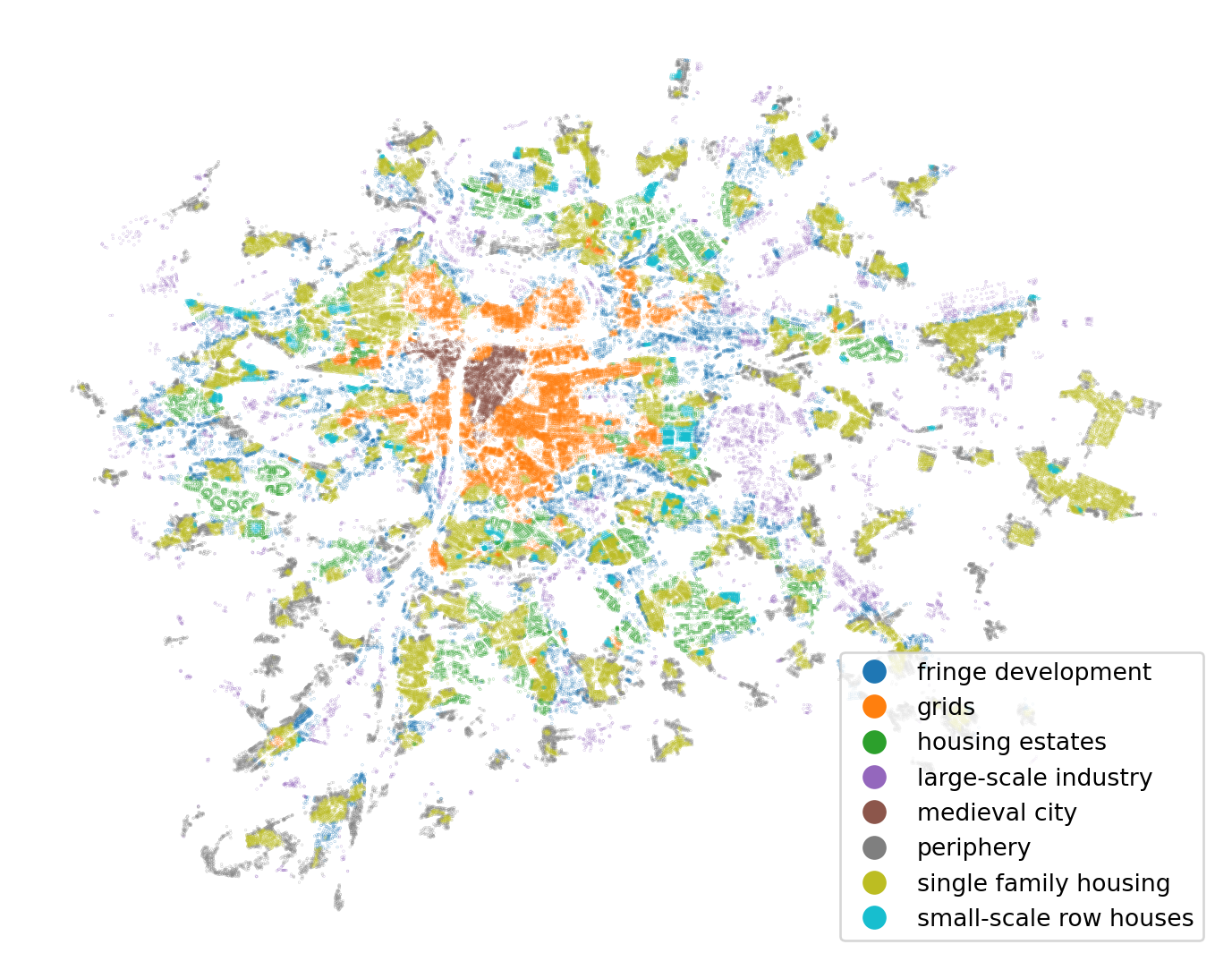
List the columns containing some numerical value and save it as a variable. There are six of them out of the original few hundred.

independent_variables = [
    "floor_area_ratio",
    "height",
    "compactness",
    "street_alignment",
    "interbuilding_distance",
    "block_perimeter_wall_length",
]

It may be helpful to understand the spatial distribution of each of them to know what to expect, and build an intuition about their relationship with the classification above.

fig, axs = plt.subplots(3, 2, figsize=(9, 9))
axs = axs.flatten()
for i, var in enumerate(independent_variables):
    building_data.plot(var, markersize=0.01, cmap="bone_r", ax=axs[i])
    axs[i].set_title(var, fontdict={"fontsize": 8})
    axs[i].set_axis_off()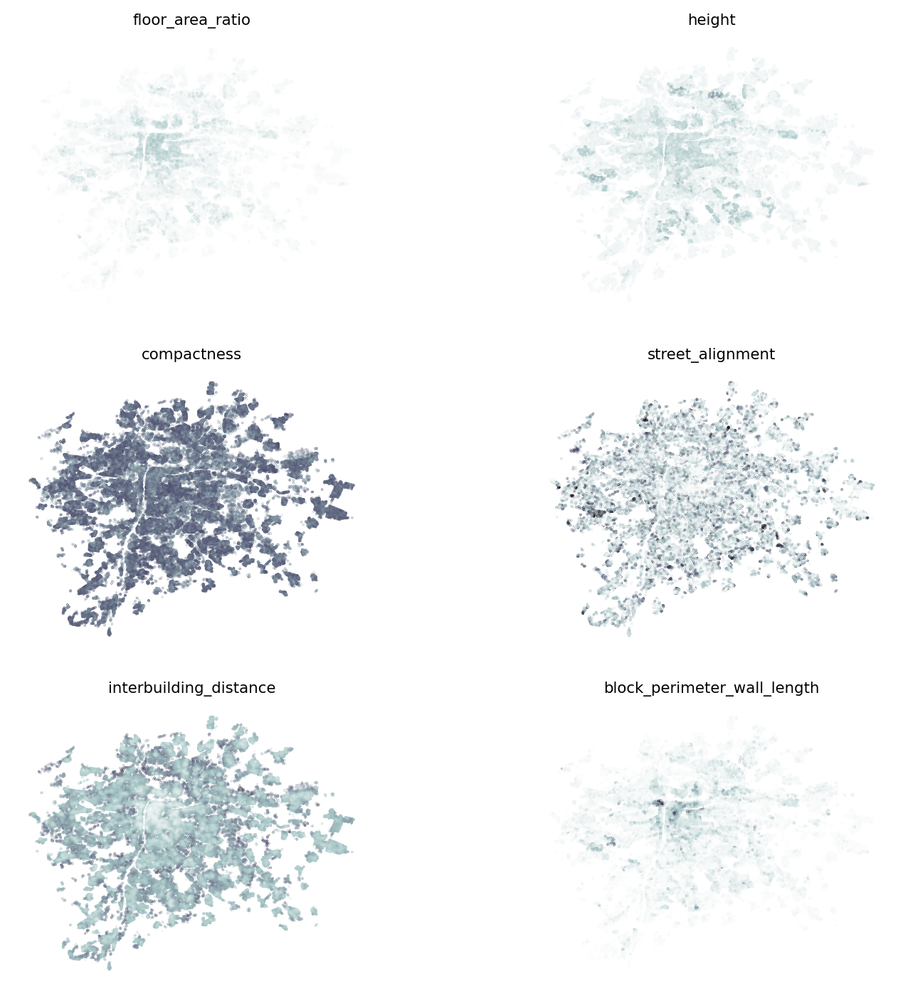

Independent (or explanatory) variables

Classification 101

The main task of today is to train classification models using the scikit-learn, so let’s begin.

Data preparation

The dataset contains a bit over 140k points. While more data tend to bring additional performance to ML models, the relationship is far from linear, and you often get nearly as performant models using just a fraction of data. Moreover, it takes longer to train on more data :).

Select a random sample of 20k points you will work with. You can later test for yourself how big of an effect the size of the sample has.

1training_sample = building_data.sample(20_000, random_state=0)

1

random_state ensures reproducibility. The sample will be the same every time.

From the sample, extract the DataFrame with just the independent variables for the simplicity.

independent = training_sample[independent_variables]
independent.head(2)

	floor_area_ratio	height	compactness	street_alignment	interbuilding_distance	block_perimeter_wall_length
34984	0.139151	4.833	0.321089	0.615831	26.019856	72.103088
39935	2.209054	20.939	0.584905	2.867204	21.971761	1107.995952

Train-test split

You already know what train-test split is from the last session. The same code used for regression can be used for classification (now).

1X_train, X_test, y_train, y_test = model_selection.train_test_split(
    independent, training_sample["cluster"], test_size=0.25, random_state=0
)

1

X and y are not very explanatory variable names but they are used in ML so often to reflect independent (X) and dependent (y) variables that everyone knows what they mean.

Random Forest Classifier

As the last time, let’s not overcomplicate your life with overview of various model architectures. The goal of today is to learn how to include the spatial dimension in them and that is the same for most of them. Pick a random forest classifier and fit the baseline model without thinking about space and geography at all.

1model = ensemble.RandomForestClassifier(random_state=0, n_jobs=-1)
2model.fit(X_train, y_train)

1

n_jobs=-1 specifies that the algorithm should use all available cores. Otherwise, it runs in a single thread only.

2

The first argument is a 2-D array of independent variables, and the second is a 1-D array of labels you want to predict.

RandomForestClassifier(n_jobs=-1, random_state=0)

In a Jupyter environment, please rerun this cell to show the HTML representation or trust the notebook.
On GitHub, the HTML representation is unable to render, please try loading this page with nbviewer.org.

Prediction

The trained model can be directly used to predict the classes (type of development in this case). Using the test portion of data, you can get the predicted label:

pred = model.predict(X_test)
pred

array(['single family housing', 'single family housing', 'medieval city',
       ..., 'single family housing', 'grids', 'single family housing'],
      dtype=object)

Or probabilities for every single class. The class prediction above just involves selecting the one with the maximum probability.

proba = model.predict_proba(X_test)
proba

array([[0.02, 0.18, 0.06, ..., 0.04, 0.42, 0.25],
       [0.01, 0.  , 0.  , ..., 0.13, 0.86, 0.  ],
       [0.  , 0.2 , 0.  , ..., 0.  , 0.  , 0.  ],
       ...,
       [0.03, 0.09, 0.  , ..., 0.07, 0.49, 0.32],
       [0.  , 0.99, 0.  , ..., 0.  , 0.  , 0.01],
       [0.07, 0.18, 0.04, ..., 0.  , 0.52, 0.09]])

Both outputs are numpy arrays, but the probabilities would be especially helpful to see as a DataFrame with column names representing class names. Those are available as .classes_:

model.classes_

array(['fringe development', 'grids', 'housing estates',
       'large-scale industry', 'medieval city', 'periphery',
       'single family housing', 'small-scale row houses'], dtype=object)

You can quickly combine it all with the original index to get a DataFrame of probabilities.

pd.DataFrame(proba, columns=model.classes_, index=X_test.index)

	fringe development	grids	housing estates	large-scale industry	medieval city	periphery	single family housing	small-scale row houses
42677	0.02	0.18	0.06	0.03	0.0	0.04	0.42	0.25
72818	0.01	0.00	0.00	0.00	0.0	0.13	0.86	0.00
8884	0.00	0.20	0.00	0.00	0.8	0.00	0.00	0.00
85469	0.25	0.00	0.01	0.01	0.0	0.10	0.63	0.00
111045	0.45	0.01	0.05	0.20	0.0	0.27	0.02	0.00
...	...	...	...	...	...	...	...	...
17114	0.60	0.00	0.06	0.07	0.0	0.21	0.06	0.00
33641	0.02	0.02	0.00	0.00	0.0	0.28	0.67	0.01
119950	0.03	0.09	0.00	0.00	0.0	0.07	0.49	0.32
22551	0.00	0.99	0.00	0.00	0.0	0.00	0.00	0.01
85085	0.07	0.18	0.04	0.10	0.0	0.00	0.52	0.09

5000 rows × 8 columns

Evaluation

Now comes the evaluation part. Normally, you are interested in a number of performance metrics capturing how good the model is. Among the most common ones are accuracy and Cohen’s kappa score. Accuracy captures the fraction of correct predictions, i.e., how many labels in the predicted array equal the known labels. Kappa score is seen as a more robust metric but not straightforwardly interpretable.

1accuracy = metrics.accuracy_score(pred, y_test)
kappa = metrics.cohen_kappa_score(pred, y_test)

summary = f"""\
Evaluation metrics
==================
Basic model:
  Accuracy: {round(accuracy, 3)}
  Kappa:    {round(kappa, 3)}
"""

2print(summary)

1

scikit-learn implements both in the metrics module.

2

Since you will need to compare many models today, let’s start building the summary using multiline f-strings.

Evaluation metrics
==================
Basic model:
  Accuracy: 0.585
  Kappa:    0.45

The results are not bad, considering the limited amount of information provided in independent variables. Around 58% of labels are correctly predicted.

Apart from the model performance, you can also evaluate how important each of the independent variables for the result is using the .feature_importances_ metric. Again, wrapping it in a pandas object is useful to get feature names alongside the values.

pd.Series(model.feature_importances_, index=model.feature_names_in_).sort_values()

compactness                    0.125213
street_alignment               0.125471
floor_area_ratio               0.166246
height                         0.174648
block_perimeter_wall_length    0.187244
interbuilding_distance         0.221179
dtype: float64

There seems to be a relatively good balance of importance ranging from 12% for compactness to 22% for inter-building distance. Check if that matches our intuition in relation to the spatial distribution of each of them.

Cross-validated prediction

To get a full map, we need to use cross-validated prediction once again. For the detailed explanation see the previous chapter on non-linear regression.

predicted = model_selection.cross_val_predict(
    model, independent, training_sample["cluster"], cv=4, n_jobs=-1
)

ax = training_sample.plot(predicted, legend=True, figsize=(9, 9), markersize=0.1)
ax.set_axis_off()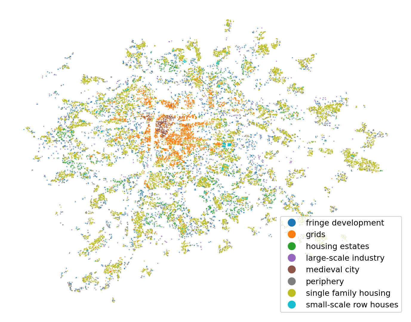

Predicted labels

What CV-prediction allows to not only plot the labels but importantly to plot the spatial pattern of errors.

ax = training_sample.plot(
    predicted == training_sample["cluster"],
    categorical=True,
    figsize=(9, 9),
    markersize=0.1,
    cmap="bwr_r",
    legend=True,
)
ax.set_axis_off()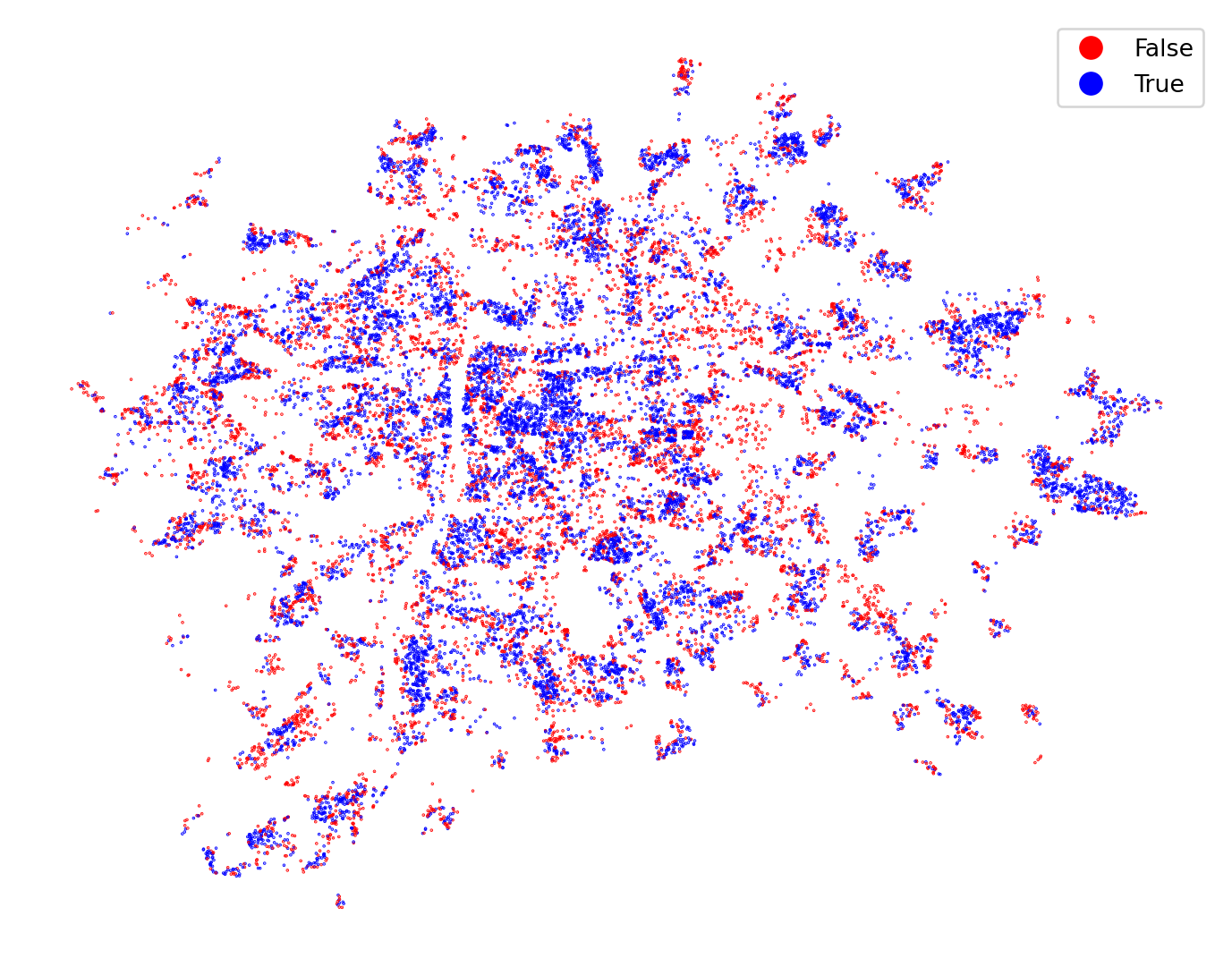

Spatial pattern of correct (True) and incorrect (False) predictions

As with the linear regression, a spatial autocorrelation of errors means that the model does not represent space reliably and may need some adaptations.

Spatial cross-validation

The same discussed in the regression chapter applies to classification. Spaital leakage caused by spatial dependency is a real problem and needs to be mitigated.

You can do that based on many criteria, but it is handy to have a variable representing those regions as the "basic_settlement_unit" column in your DataFrame.

With a categorical column indicating groups, you can use the StratifiedGroupKFold class from the scikit-learn to create the folds. Stratified K-fold not only ensures that the data is split by groups but also that there is a roughly equal proportion of classes within each split.

1gkf = model_selection.StratifiedGroupKFold(n_splits=5)
2splits = gkf.split(
    training_sample,
    training_sample.cluster,
    groups=training_sample.basic_settlement_unit,
)

1

Specify the number of folds (parts).

2

Get the iterator with different splits.

The splits variable now contains an iterator - an object we can loop through that gives you train and test parts for each split. You can easily extract the labels indicating the splits:

1split_label = np.empty(len(training_sample), dtype=float)
2for i, (train, test) in enumerate(splits):
3    split_label[test] = i
4training_sample["split"] = split_label

1

Create an empty array you will fill with the actual label using the for loop.

2

Loop over splits. Every loop gives you indices for train and test splits. You can use enumerate to get a split label.

3

Assing split labels to the subset of points used for the test in each loop.

4

Assing the labels to the DataFrame.

With the labels extracted from StratifiedGroupKFold, you can plot the splits on a map.

1ax = training_sample.plot(
  "split", categorical=True, figsize=(9, 9), markersize=0.1, legend=True
)
2training_sample.dissolve("basic_settlement_unit").convex_hull.boundary.plot(
    ax=ax, color="k", linewidth=0.5, markersize=0
)
ax.set_axis_off()

1

Plot the split labels

2

Plot the convex hull around each basic settlement unit for better visualization of regions in spatial CV.

Data splits based on spatial cross-validation

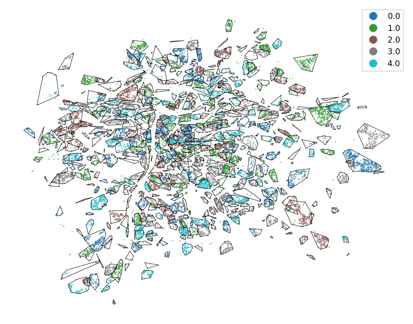
With the new, and arguably better train-test, split, you can create new training and evaluation data. You can use the split with the label 0 as a test part and the rest as a train part.

train = training_sample["split"] != 0
X_train = independent.loc[train]
y_train = training_sample["cluster"].loc[train]

test = training_sample["split"] == 0
X_test = independent.loc[test]
y_test = training_sample["cluster"].loc[test]

New data require a new model.

rf_spatial_cv = ensemble.RandomForestClassifier(random_state=0, n_jobs=-1)
rf_spatial_cv.fit(X_train, y_train)

RandomForestClassifier(n_jobs=-1, random_state=0)

In a Jupyter environment, please rerun this cell to show the HTML representation or trust the notebook.
On GitHub, the HTML representation is unable to render, please try loading this page with nbviewer.org.

And its evaluation. Just use += to add to the existing summary.

pred = rf_spatial_cv.predict(X_test)

accuracy_spatial_cv = metrics.accuracy_score(pred, y_test)
kappa_spatial_cv = metrics.cohen_kappa_score(pred, y_test)

summary += f"""\
Basic model with spatial cross-validation:
  Accuracy: {round(accuracy_spatial_cv, 3)}
  Kappa:    {round(kappa_spatial_cv, 3)}
"""

print(summary)

Evaluation metrics
==================
Basic model:
  Accuracy: 0.585
  Kappa:    0.45
Basic model with spatial cross-validation:
  Accuracy: 0.57
  Kappa:    0.419

The results are marginally worse, but that is expected. It means that the original model was indeed a bit leaking! The model based on the spatial CV should be more robust than the previous one, meaning that it should perform as expected on unseen data.

The result is worse on paper but is now more spatially robust - it will generalize better on unseen data.

Feature engineering

Sometimes, the original data is just not enough for a decent prediction. At that point, you may want to include some other variables that would help, but they may not be readily available, and you need to create them.

The first option is to look at the data you have and extract some additional information from it using methods known as map synthesis.

Map synthesis

Map synthesis uses the spatial structure of the data to derive new features. There’s no external input, you simply put geography at work.

Point density

There are methods of map synthesis that work directly with existing values, and there are those that look solely at the spatial distribution of your data. One example of the latter is a measurement of point density (number of neighbors within a distance band).

You should already know how to do that using the graph module of libpysal. Create a Graph and extract its cardinalities (the number of neighbors).

distance_200 = graph.Graph.build_distance_band(training_sample, 200)
training_sample["points_in_200m"] = distance_200.cardinalities

Let’s check if the result has some meaningful spatial pattern.

ax = training_sample.plot("points_in_200m", figsize=(9, 9), markersize=0.1)
ax.set_axis_off()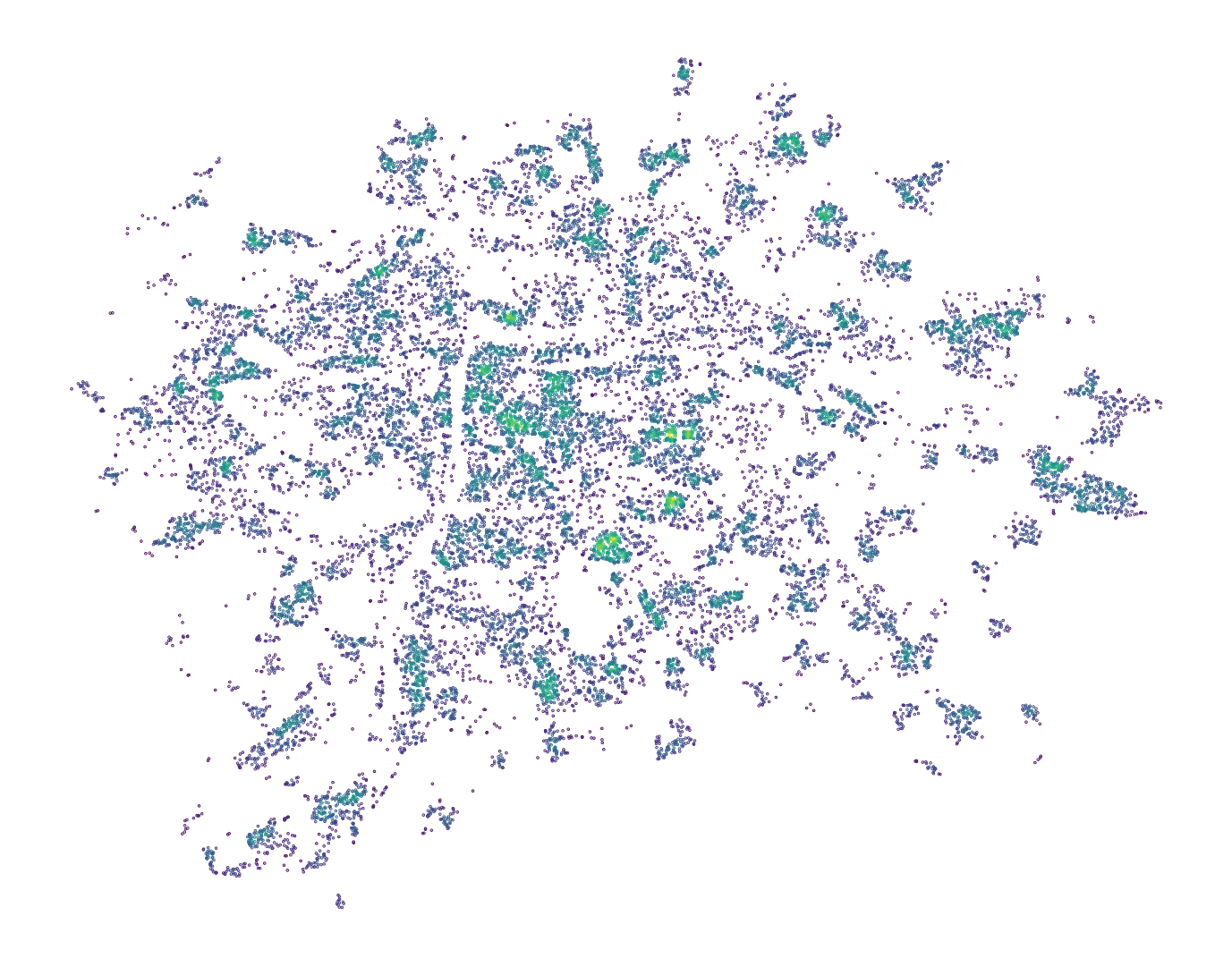

Point density within a 200m distance band

It is not a strong one, but there are clear pockets of the higher point density, so this new column can help with the prediction accuracy. Create a new set of independent variables, including the new one, and generate new training and evaluation data.

independent_proximity = training_sample[
1    independent_variables + ["points_in_200m"]
]

X_train = independent_proximity.loc[train]
y_train = training_sample["cluster"].loc[train]

X_test = independent_proximity.loc[test]
y_test = training_sample["cluster"].loc[test]

1

Add the new column to the list of existing columns and use it to subset the DataFrame.

The rest is simply rinse and repeat. Create the model and train it on new data.

rf_proximity = ensemble.RandomForestClassifier(random_state=0, n_jobs=-1)
rf_proximity.fit(X_train, y_train)

RandomForestClassifier(n_jobs=-1, random_state=0)

In a Jupyter environment, please rerun this cell to show the HTML representation or trust the notebook.
On GitHub, the HTML representation is unable to render, please try loading this page with nbviewer.org.

And evaluate it in the same way as before.

pred = rf_proximity.predict(X_test)

accuracy_proximity = metrics.accuracy_score(pred, y_test)
kappa_proximity = metrics.cohen_kappa_score(pred, y_test)

summary += f"""\
Points within 200m (spatial CV):
  Accuracy: {round(accuracy_proximity, 3)}
  Kappa:    {round(kappa_proximity, 3)}
"""
print(summary)

Evaluation metrics
==================
Basic model:
  Accuracy: 0.585
  Kappa:    0.45
Basic model with spatial cross-validation:
  Accuracy: 0.57
  Kappa:    0.419
Points within 200m (spatial CV):
  Accuracy: 0.598
  Kappa:    0.46

Remember that your baseline model is the Basic model with spatial cross-validation. Compared to that, the performance of the new model is a bit better, especially when looking at Cohen’s kappa. It seems that the point density brings some value. You can check how important it is compared to the original variables.

pd.Series(
    rf_proximity.feature_importances_, index=rf_proximity.feature_names_in_
).sort_values()

compactness                    0.108827
street_alignment               0.109489
points_in_200m                 0.126702
floor_area_ratio               0.146121
height                         0.159027
block_perimeter_wall_length    0.173754
interbuilding_distance         0.176080
dtype: float64

It seems that not that much, but each percent of accuracy counts.

Point density is just one example, and there are many more. Below, when dealing with spatial dependence, you’ll get back to map synthesis once again. But before that, let’s use some external data to improve the model.

Proximity variables

Sometimes, you may have an assumption that a distance to a specific location or a set of locations makes a difference to the spatial distribution of the dependent variable, and the inclusion of a variable reflecting this distance could help the model. You can think of distance to subway stations when dealing with rent price prediction or distance to highways when trying to predict air pollution. In the case of urban development in Prague, it may be interesting to capture the distance from the city centre. Prague is a very monocentric city whose development happened over the years in a series of concentric rings. First, the medieval centre, then industrial-era neighborhoods behind the original city walls, and so on. Therefore, a distance to Old Town Square may be useful for the development type prediction.

You have done this before, so fire up geocoding, and extract the point representing the square in the same CRS the rest of the data is in.

old_town_square = (
    gpd.tools.geocode("Old Town Square, Prague")
    .to_crs(building_data.crs)
    .geometry.item()
)

With the point, you can measure the distance from every building in the training sample and use the resulting column as another independent variable.

training_sample["distance_to_old_town"] = training_sample.distance(old_town_square)

ax = training_sample.plot("distance_to_old_town", figsize=(9, 9), markersize=0.1)
ax.set_axis_off()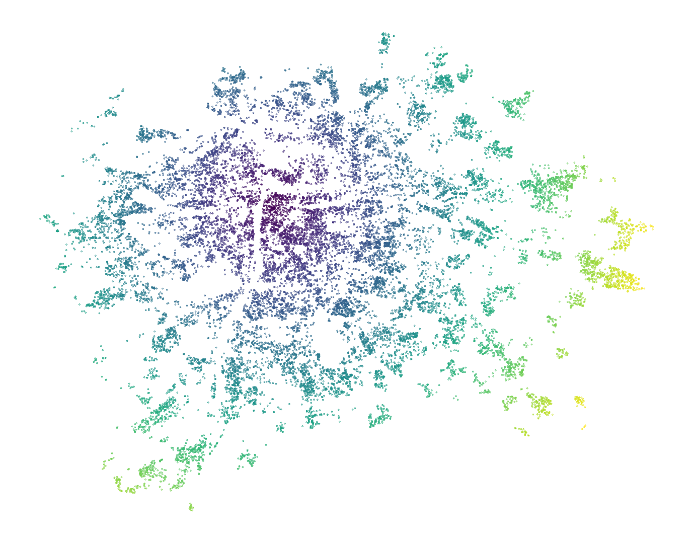

Distance to the Old Town Square

Now simply add it to the DataFrame representing independent variables and the rest is the same.

independent_distance = training_sample[
    independent_variables + ["points_in_200m", "distance_to_old_town"]
]

X_train = independent_distance.loc[train]
y_train = training_sample["cluster"].loc[train]

X_test = independent_distance.loc[test]
y_test = training_sample["cluster"].loc[test]

Get a new, hopefully better model.

rf_distance = ensemble.RandomForestClassifier(random_state=0, n_jobs=-1)
rf_distance.fit(X_train, y_train)

RandomForestClassifier(n_jobs=-1, random_state=0)

In a Jupyter environment, please rerun this cell to show the HTML representation or trust the notebook.
On GitHub, the HTML representation is unable to render, please try loading this page with nbviewer.org.

And check if the new variable makes a difference.

pred = rf_distance.predict(X_test)

accuracy_distance = metrics.accuracy_score(pred, y_test)
kappa_distance = metrics.cohen_kappa_score(pred, y_test)

summary += f"""\
Distance to Old Town Sq + above (spatial CV):
  Accuracy: {round(accuracy_distance, 3)}
  Kappa:    {round(kappa_distance, 3)}
"""
print(summary)

Evaluation metrics
==================
Basic model:
  Accuracy: 0.585
  Kappa:    0.45
Basic model with spatial cross-validation:
  Accuracy: 0.57
  Kappa:    0.419
Points within 200m (spatial CV):
  Accuracy: 0.598
  Kappa:    0.46
Distance to Old Town Sq + above (spatial CV):
  Accuracy: 0.651
  Kappa:    0.532

That is quite a decent bump in performance! It seems that the distance to the city centre is not bad in explaining the development typology. Check how important it is within the model.

pd.Series(
    rf_distance.feature_importances_, index=rf_distance.feature_names_in_
).sort_values()

compactness                    0.083833
street_alignment               0.084431
points_in_200m                 0.114884
floor_area_ratio               0.118693
height                         0.121907
block_perimeter_wall_length    0.136004
interbuilding_distance         0.143222
distance_to_old_town           0.197027
dtype: float64

Interestingly enough, it seems to be more explanatory than any of the variables reflecting the actual morphology.

Map matching

In other cases, you can make use of other data and link it to existing data. When you join the data based on spatial operation, you can talk about map matching. You can measure a number of points of interest in the vicinity of each location, link the data from rasters, interpolate them from point patterns or from polygons to other polygons. By now, you should know all that, so there’s no need to go into detail. Sticking to a simple case, map matching can also be done using a spatial join.

Load the price data you worked with in the Learning GeoPandas chapter.

price = gpd.read_file(
    "https://martinfleischmann.net/sds/geographic_data/data/SED_CenovaMapa_p_shp.zip",
)
1price["CENA"] = price["CENA"].replace("N", None).astype("float")
price.head(2)

1

Price is in the column called "CENA", which needs to be turned to floats.

	KOD_UNI	MAPA	STRED	CENA	FUNKCE	TYP_CENY	zmena	Shape_Leng	Shape_Area	geometry
0	11	4	0	7100.0	R2	181920-pary	0	2032.256585	82031.672127	POLYGON Z ((-737015.74 -1034316.4 0, -737018.2...
1	10921	4	0	9030.0	R1	181920-pary	0	450.070407	11837.482327	POLYGON Z ((-737103.202 -1034331.743 0, -73710...

Before any spatial joins, check the CRS.

price.crs.equals(training_sample.crs)

False

And, like in this case, don’t forget to re-project geometries in case of a CRS mismatch. Then you can go ahead with the spatial join.

price = price.to_crs(training_sample.crs)

training_sample_price = training_sample.sjoin(
1    price[["CENA", "geometry"]].dropna()
)
training_sample_price.head(2)

1

Ignore rows with missing prices, as those will bring no value, only issues.

	cluster	floor_area_ratio	height	compactness	street_alignment	interbuilding_distance	block_perimeter_wall_length	basic_settlement_unit	cadastral zone	geometry	split	points_in_200m	distance_to_old_town	index_right	CENA
34984	single family housing	0.139151	4.833	0.321089	0.615831	26.019856	72.103088	Běchovice	Běchovice	POINT (-728888.096 -1045720.683)	1.0	7	14202.783900	4769	7100.0
39935	grids	2.209054	20.939	0.584905	2.867204	21.971761	1107.995952	Na Pankráci	Nusle	POINT (-742882.423 -1046165.913)	0.0	23	3155.348653	5033	12720.0

You can prepare data for a model with price included.

independent_proximity_price = training_sample_price[
    independent_variables + ["points_in_200m", "distance_to_old_town", "CENA"]
]

1train_price = training_sample_price["split"] != 0
X_train = independent_proximity_price.loc[train_price]
y_train = training_sample_price["cluster"].loc[train_price]

test_price = training_sample_price["split"] == 0
X_test = independent_proximity_price.loc[test_price]
y_test = training_sample_price["cluster"].loc[test_price]

1

Get the new split mask as due to some points not being merged to any geometries, training_sample_price is slightly shorter than training_sample, and the original mask does not align.

The rest, you know. First the model.

rf_distance_price = ensemble.RandomForestClassifier(random_state=0, n_jobs=-1)
rf_distance_price.fit(X_train, y_train)

RandomForestClassifier(n_jobs=-1, random_state=0)

In a Jupyter environment, please rerun this cell to show the HTML representation or trust the notebook.
On GitHub, the HTML representation is unable to render, please try loading this page with nbviewer.org.

Then, the evaluation.

pred = rf_distance_price.predict(X_test)

accuracy_distance_price = metrics.accuracy_score(pred, y_test)
kappa_distance_price = metrics.cohen_kappa_score(pred, y_test)

summary += f"""\
Price + above (spatial CV):
  Accuracy: {round(accuracy_distance_price, 3)}
  Kappa:    {round(kappa_distance_price, 3)}
"""
print(summary)

Evaluation metrics
==================
Basic model:
  Accuracy: 0.585
  Kappa:    0.45
Basic model with spatial cross-validation:
  Accuracy: 0.57
  Kappa:    0.419
Points within 200m (spatial CV):
  Accuracy: 0.598
  Kappa:    0.46
Distance to Old Town Sq + above (spatial CV):
  Accuracy: 0.651
  Kappa:    0.532
Price + above (spatial CV):
  Accuracy: 0.673
  Kappa:    0.553

Another improvement. It seems that price is not that critical, but is surely brings some value.

pd.Series(
    rf_distance_price.feature_importances_, index=rf_distance_price.feature_names_in_
).sort_values()

compactness                    0.065115
street_alignment               0.066357
floor_area_ratio               0.086397
points_in_200m                 0.103891
height                         0.111930
interbuilding_distance         0.119208
CENA                           0.136275
block_perimeter_wall_length    0.139565
distance_to_old_town           0.171261
dtype: float64

As the feature importance shows, it is among the most important variables, though the distance to the Old Town Sq. is still unbeaten.

Spatial dependence

Let’s get back to map synthesis and talk about spatial dependence. Some phenomena, urban development type may be one of them, are not explained only by values linked to individual geometries but also by the spatial configuration of the observations around. If the mean inter-building distance of observation A is small but that of nearly all observations around is high, it may be worth taking that into account. You can say that the predicted value on observation A depends on the spatial context and configuration around it. Generally speaking, the values of observations are related to each other based on their distance and are spatially dependent, reflecting Tobler’s First law of geography once again.

Include spatially lagged variables in the model

The simplest way of incorporating spatial dependence to a generic ML model is to add variables to your set of independent variables capturing spatial dependence through spatial lag.

Use the spatial weights matrix created above and generate a spatial lag of all independent variables.

1distance_200_row = distance_200.transform("r")
2lagged_variables = []
3for var in independent_variables:
4    training_sample[f"{var}_lag"] = distance_200_row.lag(training_sample[var])
5    lagged_variables.append(f"{var}_lag")
training_sample.head(2)

1

Remember that the graph needs to be row-standardised to get a mean value.

2

Create and empty list that will be populated with names of new lagged variables.

3

Loop through the list of existing independent variables.

4

Measure a lag for each and assign it to a column.

5

Add the name to the list.

	cluster	floor_area_ratio	height	compactness	street_alignment	interbuilding_distance	block_perimeter_wall_length	basic_settlement_unit	cadastral zone	geometry	split	points_in_200m	distance_to_old_town	floor_area_ratio_lag	height_lag	compactness_lag	street_alignment_lag	interbuilding_distance_lag	block_perimeter_wall_length_lag
34984	single family housing	0.139151	4.833	0.321089	0.615831	26.019856	72.103088	Běchovice	Běchovice	POINT (-728888.096 -1045720.683)	1.0	7	14202.783900	0.199820	5.657571	0.546654	5.776773	23.220023	58.535778
39935	grids	2.209054	20.939	0.584905	2.867204	21.971761	1107.995952	Na Pankráci	Nusle	POINT (-742882.423 -1046165.913)	0.0	23	3155.348653	1.281836	14.360696	0.539464	3.990104	21.274888	324.468169

It may be interesting to assess the effect of spatial dependence without the variables added above. Combine original independent variables with the new lagged and prepare new training data.

independent_lag = training_sample[independent_variables + lagged_variables]

X_train = independent_lag.loc[train]
y_train = training_sample["cluster"].loc[train]

X_test = independent_lag.loc[test]
y_test = training_sample["cluster"].loc[test]

Fit the new model, which should be able to use spatial dependence.

rf_lag_200m = ensemble.RandomForestClassifier(random_state=0, n_jobs=-1)
rf_lag_200m.fit(X_train, y_train)

RandomForestClassifier(n_jobs=-1, random_state=0)

In a Jupyter environment, please rerun this cell to show the HTML representation or trust the notebook.
On GitHub, the HTML representation is unable to render, please try loading this page with nbviewer.org.

And check how significant an effect it has on the model performance.

pred = rf_lag_200m.predict(X_test)

accuracy_lag = metrics.accuracy_score(pred, y_test)
kappa_lag = metrics.cohen_kappa_score(pred, y_test)

summary += f"""\
Spatial dependence - lagged model (spatial CV):
  Accuracy: {round(accuracy_lag, 3)}
  Kappa:    {round(kappa_lag, 3)}
"""
print(summary)

Evaluation metrics
==================
Basic model:
  Accuracy: 0.585
  Kappa:    0.45
Basic model with spatial cross-validation:
  Accuracy: 0.57
  Kappa:    0.419
Points within 200m (spatial CV):
  Accuracy: 0.598
  Kappa:    0.46
Distance to Old Town Sq + above (spatial CV):
  Accuracy: 0.651
  Kappa:    0.532
Price + above (spatial CV):
  Accuracy: 0.673
  Kappa:    0.553
Spatial dependence - lagged model (spatial CV):
  Accuracy: 0.678
  Kappa:    0.573

That is surely not negligible, considering that no other data were needed.

pd.Series(
    rf_lag_200m.feature_importances_, index=rf_lag_200m.feature_names_in_
).sort_values()

compactness                        0.043229
street_alignment                   0.046029
height                             0.057588
floor_area_ratio                   0.058145
block_perimeter_wall_length        0.067363
street_alignment_lag               0.070991
compactness_lag                    0.075911
height_lag                         0.102984
interbuilding_distance             0.103224
interbuilding_distance_lag         0.114796
block_perimeter_wall_length_lag    0.126160
floor_area_ratio_lag               0.133580
dtype: float64

The feature importance very clearly shows that when detecting urban typology, the context is always more important than the individual observation. It is expected as the typology attempts to reflect the general pattern of development but you can see the similar effect in many other situations.

Spatial heterogneity

While ML models like the random forest learn interaction between variables, they are not always able to pick up spatial heterogeneity of the interaction between dependent and independent variables. Last week, you tried to deal with spatial heterogeneity using the categorical variable reflecting the spatial fixed effect. You could do the same here, but let’s try another approach.

Include x, y coordinates

Including the x and y (or longitude and latitude) coordinates of your geometries is a clever way of capturing the spatial heterogeneity in the model. The location serves as a proxy for any unexplained variance of a spatial nature. It does not help you with interpretation, as coordinates do not explain anything.

The model will also struggle to generalise outside of the original spatial extent. So while a model trained on Prague using the original set of variables could be easily used in any other Czech city, like Brno, the model that includes coordinates would have no idea how to interpret the values it would see in Brno. Use with caution.

Technically, it is dead simple. You just include coordinates as another two columns.

training_sample[["x", "y"]] = training_sample.get_coordinates()
training_sample.head(2)

	cluster	floor_area_ratio	height	compactness	street_alignment	interbuilding_distance	block_perimeter_wall_length	basic_settlement_unit	cadastral zone	geometry	...	points_in_200m	distance_to_old_town	floor_area_ratio_lag	height_lag	compactness_lag	street_alignment_lag	interbuilding_distance_lag	block_perimeter_wall_length_lag	x	y
34984	single family housing	0.139151	4.833	0.321089	0.615831	26.019856	72.103088	Běchovice	Běchovice	POINT (-728888.096 -1045720.683)	...	7	14202.783900	0.199820	5.657571	0.546654	5.776773	23.220023	58.535778	-728888.096013	-1.045721e+06
39935	grids	2.209054	20.939	0.584905	2.867204	21.971761	1107.995952	Na Pankráci	Nusle	POINT (-742882.423 -1046165.913)	...	23	3155.348653	1.281836	14.360696	0.539464	3.990104	21.274888	324.468169	-742882.423186	-1.046166e+06

2 rows × 21 columns

To check the effect of spatial heterogeneity compared to the baseline model, create new training data with the original variables and coordinates on top.

independent_coordinates = training_sample[independent_variables + ["x", "y"]]

X_train = independent_coordinates.loc[train]
y_train = training_sample["cluster"].loc[train]

X_test = independent_coordinates.loc[test]
y_test = training_sample["cluster"].loc[test]

Train the model.

rf_coordinates = ensemble.RandomForestClassifier(random_state=0, n_jobs=-1)
rf_coordinates.fit(X_train, y_train)

RandomForestClassifier(n_jobs=-1, random_state=0)

In a Jupyter environment, please rerun this cell to show the HTML representation or trust the notebook.
On GitHub, the HTML representation is unable to render, please try loading this page with nbviewer.org.

And evaluate its performance.

pred = rf_coordinates.predict(X_test)

accuracy_coordinates = metrics.accuracy_score(pred, y_test)
kappa_coordinates = metrics.cohen_kappa_score(pred, y_test)

summary += f"""\
Spatial heterogeneity - coordinates (spatial CV):
  Accuracy: {round(accuracy_coordinates, 3)}
  Kappa:    {round(kappa_coordinates, 3)}
"""
print(summary)

Evaluation metrics
==================
Basic model:
  Accuracy: 0.585
  Kappa:    0.45
Basic model with spatial cross-validation:
  Accuracy: 0.57
  Kappa:    0.419
Points within 200m (spatial CV):
  Accuracy: 0.598
  Kappa:    0.46
Distance to Old Town Sq + above (spatial CV):
  Accuracy: 0.651
  Kappa:    0.532
Price + above (spatial CV):
  Accuracy: 0.673
  Kappa:    0.553
Spatial dependence - lagged model (spatial CV):
  Accuracy: 0.678
  Kappa:    0.573
Spatial heterogeneity - coordinates (spatial CV):
  Accuracy: 0.632
  Kappa:    0.501

There indeed is some degree of spatial heterogeneity, but its effect is not that strong as that of spatial dependence.

pd.Series(
    rf_coordinates.feature_importances_, index=rf_coordinates.feature_names_in_
).sort_values()

compactness                    0.079772
street_alignment               0.082567
height                         0.120324
floor_area_ratio               0.121949
block_perimeter_wall_length    0.140227
x                              0.141132
y                              0.144687
interbuilding_distance         0.169343
dtype: float64

Interpreting feature importance is a bit more complicated, as x and y are not to be treated as two separate variables but as a pair. You can try to sum their importance, but remember that the result may be misleading.

Heterogeneity and dependence

You can try to combine the effects of heterogeneity and dependence within a single model as each seems to help when used separately.

independent_coordinates = training_sample[
    independent_variables + lagged_variables + ["x", "y"]
]

X_train = independent_coordinates.loc[train]
y_train = training_sample["cluster"].loc[train]

X_test = independent_coordinates.loc[test]
y_test = training_sample["cluster"].loc[test]

Let’s consider this a final model of the day.

rf_het_dep = ensemble.RandomForestClassifier(random_state=0, n_jobs=-1)
rf_het_dep.fit(X_train, y_train)

RandomForestClassifier(n_jobs=-1, random_state=0)

In a Jupyter environment, please rerun this cell to show the HTML representation or trust the notebook.
On GitHub, the HTML representation is unable to render, please try loading this page with nbviewer.org.

The final evaluation:

pred = rf_het_dep.predict(X_test)

accuracy_het_dep = metrics.accuracy_score(pred, y_test)
kappa_het_dep = metrics.cohen_kappa_score(pred, y_test)

summary += f"""\
Spatial dependence + heterogeneity (spatial CV):
  Accuracy: {round(accuracy_het_dep, 3)}
  Kappa:    {round(kappa_het_dep, 3)}
"""
print(summary)

Evaluation metrics
==================
Basic model:
  Accuracy: 0.585
  Kappa:    0.45
Basic model with spatial cross-validation:
  Accuracy: 0.57
  Kappa:    0.419
Points within 200m (spatial CV):
  Accuracy: 0.598
  Kappa:    0.46
Distance to Old Town Sq + above (spatial CV):
  Accuracy: 0.651
  Kappa:    0.532
Price + above (spatial CV):
  Accuracy: 0.673
  Kappa:    0.553
Spatial dependence - lagged model (spatial CV):
  Accuracy: 0.678
  Kappa:    0.573
Spatial heterogeneity - coordinates (spatial CV):
  Accuracy: 0.632
  Kappa:    0.501
Spatial dependence + heterogeneity (spatial CV):
  Accuracy: 0.711
  Kappa:    0.615

This seems to be the best model so far. Keep in mind that variables coming from the feature engineering section are not included here, so there still may be some space for an improvement.

pd.Series(
    rf_het_dep.feature_importances_, index=rf_het_dep.feature_names_in_
).sort_values()

compactness                        0.032525
street_alignment                   0.036007
floor_area_ratio                   0.047823
height                             0.049390
street_alignment_lag               0.057048
block_perimeter_wall_length        0.057807
compactness_lag                    0.063732
y                                  0.068235
x                                  0.071409
height_lag                         0.083217
interbuilding_distance             0.090460
interbuilding_distance_lag         0.102752
block_perimeter_wall_length_lag    0.117814
floor_area_ratio_lag               0.121782
dtype: float64

Both lagged variables and coordinates are valuable here but keep in mind that the strength of these effects will vary dependning on specific use case. What is clearly useful in this case may have no value in other situations.

Prediction on the whole dataset

If you consider rf_het_dep a final model you are happy with, you can check how it performs on the full dataset, not only on the sample of 20k observations used above.

First, you will need all the variables computed for the full dataset.

distance_200_all = graph.Graph.build_distance_band(building_data, 200).transform("r")
for var in independent_variables:
    building_data[f"{var}_lag"] = distance_200_all.lag(building_data[var])

building_data[["x", "y"]] = building_data.get_coordinates()

Then, you can use the model for inference. First, check the probabilities.

probabilities = rf_het_dep.predict_proba(
    building_data[independent_variables + lagged_variables + ["x", "y"]]
)
probabilities

array([[0.29, 0.05, 0.42, ..., 0.  , 0.05, 0.  ],
       [0.  , 0.04, 0.  , ..., 0.  , 0.  , 0.  ],
       [0.1 , 0.  , 0.  , ..., 0.49, 0.41, 0.  ],
       ...,
       [0.  , 1.  , 0.  , ..., 0.  , 0.  , 0.  ],
       [0.  , 1.  , 0.  , ..., 0.  , 0.  , 0.  ],
       [0.52, 0.06, 0.01, ..., 0.1 , 0.07, 0.01]])

Plotting class-based probabilities allows you to visualise the likelihood that each observation (building in our case) belonging to each class.

fig, axs = plt.subplots(4, 2, figsize=(9, 14))
axs = axs.flatten()
for i, ax in enumerate(axs):
    building_data.plot(
      probabilities[:, i], markersize=0.01, cmap="bone_r", ax=ax, vmin=0, vmax=1,
    )
    axs[i].set_title(rf_het_dep.classes_[i], fontdict={"fontsize": 8})
    ax.set_axis_off()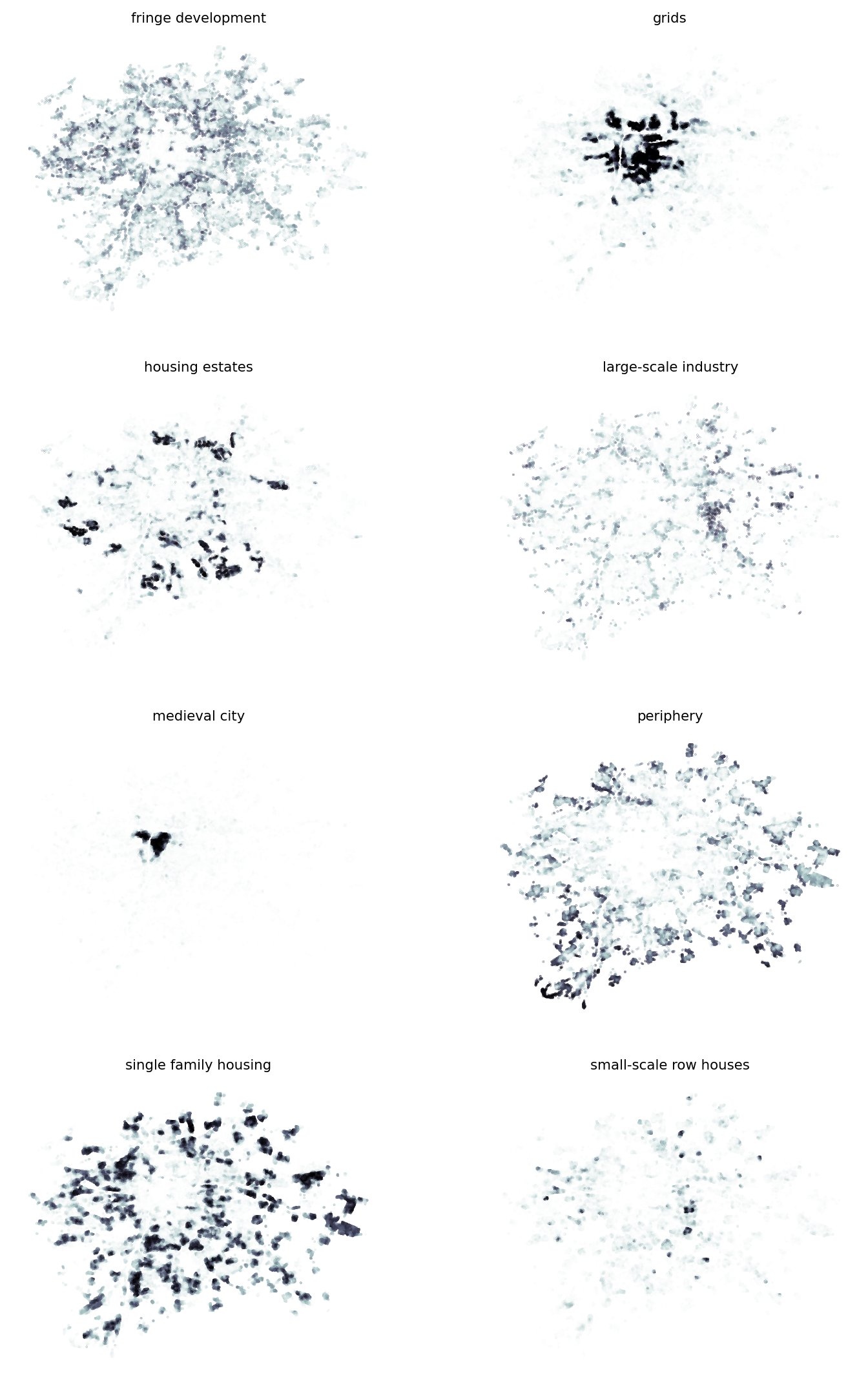

Class-based probability

Plotting the maximum probability assigned to an observation regardless of class is also useful. This can be seen as a proxy of the certainty of a model and allows you to identify areas where the model works well and has no issue picking up the correct class and those where it struggles.

building_data.plot(
    probabilities.max(axis=1), markersize=0.01, cmap="cividis_r", figsize=(9, 9)
).set_axis_off()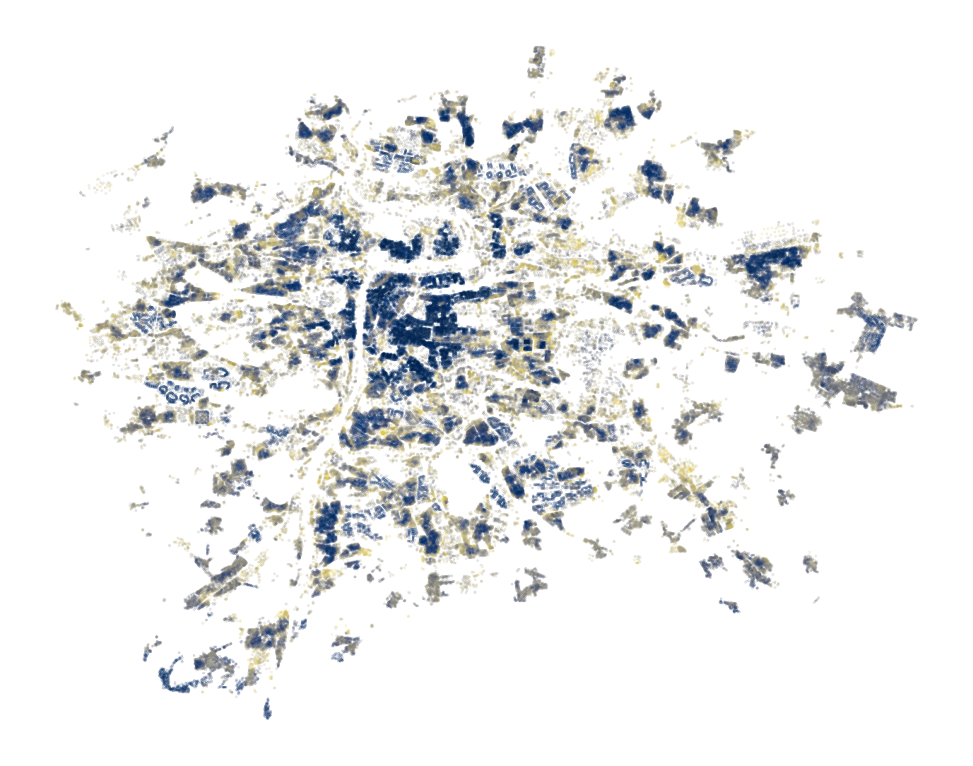

Maximum probability reflecting the certainty of the model

If you want just a label, it is easier to use the predict() method instead.

predicted_class = rf_het_dep.predict(
    building_data[independent_variables + lagged_variables + ["x", "y"]]
)

The predicted labels allow you to check the spatial pattern of errors as you did earlier.

building_data.plot(
    predicted_class == building_data["cluster"],
    categorical=True,
    figsize=(9, 9),
    markersize=0.005,
    cmap="bwr_r",
    legend=True,
).set_axis_off()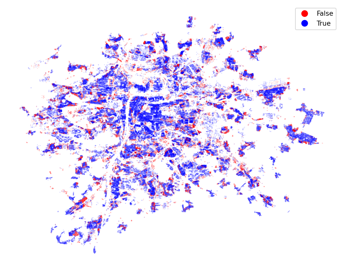

Spatial pattern of correct (True) and incorrect (False) predictions on the full dataset

Finally, you may be interested in the performance of the model on the full dataset.

accuracy_all = metrics.accuracy_score(predicted_class, building_data["cluster"])
kappa_all = metrics.cohen_kappa_score(predicted_class, building_data["cluster"])

summary += f"""
Complete dataset
----------------
Spatial dependence + heterogeneity (spatial CV):
  Accuracy: {round(accuracy_all, 3)}
  Kappa:    {round(kappa_all, 3)}
"""
print(summary)

Evaluation metrics
==================
Basic model:
  Accuracy: 0.585
  Kappa:    0.45
Basic model with spatial cross-validation:
  Accuracy: 0.57
  Kappa:    0.419
Points within 200m (spatial CV):
  Accuracy: 0.598
  Kappa:    0.46
Distance to Old Town Sq + above (spatial CV):
  Accuracy: 0.651
  Kappa:    0.532
Price + above (spatial CV):
  Accuracy: 0.673
  Kappa:    0.553
Spatial dependence - lagged model (spatial CV):
  Accuracy: 0.678
  Kappa:    0.573
Spatial heterogeneity - coordinates (spatial CV):
  Accuracy: 0.632
  Kappa:    0.501
Spatial dependence + heterogeneity (spatial CV):
  Accuracy: 0.711
  Kappa:    0.615

Complete dataset
----------------
Spatial dependence + heterogeneity (spatial CV):
  Accuracy: 0.776
  Kappa:    0.703

Not bad at all. More than 75% of buildings were correctly classified using only the data you were given in the beginning and geography. Just note that since the evaluation based on the full dataset is done based on a different sample of data than all those above, the values are not entirely comparable.

Additional reading

This material combines components from the chapters on Spatial Regression and Spatial Feature Engineering from the Geographic Data Science with Python by Rey, Arribas-Bel, and Wolf (2023).

The end

Thank you for getting this far.

References

Fleischmann, Martin, Alessandra Feliciotti, Ombretta Romice, and Sergio Porta. 2022. “Methodological Foundation of a Numerical Taxonomy of Urban Form.” Environment and Planning B: Urban Analytics and City Science 49 (4): 1283–99. https://doi.org/10/gnth7q.

Rey, Sergio, Dani Arribas-Bel, and Levi John Wolf. 2023. Geographic Data Science with Python. Chapman & Hall/CRC Texts in Statistical Science. London, England: Taylor & Francis.