Spatial weights in PySAL

In this session, you will be learning the ins and outs of one of the key pieces in spatial analysis: spatial weights matrices. These are structured sets of numbers that formalise geographical relationships between the observations in a dataset. Essentially, a spatial weights matrix of a given geography is a positive definite matrix of dimensions \(N\) by \(N\), where \(N\) is the total number of observations:

\[ W = \left(\begin{array}{cccc} 0 & w_{12} & \dots & w_{1N} \\ w_{21} & \ddots & w_{ij} & \vdots \\ \vdots & w_{ji} & 0 & \vdots \\ w_{N1} & \dots & \dots & 0 \end{array} \right) \]

where each cell \(w_{ij}\) contains a value that represents the degree of spatial contact or interaction between observations \(i\) and \(j\). A fundamental concept in this context is that of neighbour and neighbourhood. By convention, elements in the diagonal (\(w_{ii}\)) are set to zero. A neighbour of a given observation \(i\) is another observation with which \(i\) has some degree of connection. In terms of \(W\), \(i\) and \(j\) are thus neighbors if \(w_{ij} > 0\). Following this logic, the neighbourhood of \(i\) will be the set of observations in the system with which it has a certain connection or those observations with a weight greater than zero.

There are several ways to create such matrices and many more to transform them so they contain an accurate representation that aligns with the way you understand spatial interactions between the elements of a system. This session will introduce the most commonly used ones and show how to compute them with PySAL.

1import matplotlib.pyplot as plt
import contextily
import geopandas as gpd
import numpy as np
import pandas as pd
import seaborn as sns

from libpysal import graph

1: A common standard is to do all the imports on top of your notebook.

Data

For this tutorial, you will use a dataset of Basic Settlement Units (ZSJ) in Prague for 2021. The table is available as part of this course, so it can be accessed remotely through the web. If you want to see how the table was created, a notebook is available here.

To make things easier, you will read data from a file posted online so, for now, you do not need to download any dataset:

prague = gpd.read_file(
    "https://martinfleischmann.net/sds/spatial_graphs/data/zsj_prague_2021.gpkg"
)
1prague = prague.set_index("NAZ_ZSJ")
prague.explore()

1: Use the name of each observation as an index. It will help you link them to the weights matrix.

Make this Notebook Trusted to load map: File -> Trust Notebook

Alternative

Instead of reading the file directly off the web, it is possible to download it manually, store it on your computer, and read it locally. To do that, you can follow these steps:

Download the file by right-clicking on this link and saving the file
Place the file in the same folder as the notebook where you intend to read it
Replace the code in the cell above with:

prague = gpd.read_file(
    "zsj_prague_2021.gpkg",
)

Building spatial weights in `PySAL`

Contiguity

Contiguity weights matrices define spatial connections through the existence of shared boundaries. This makes it directly suitable to use with polygons: if two polygons share boundaries to some degree, they will be labelled as neighbours under these kinds of weights. Exactly how much they need to share is what differentiates the two approaches we will learn: Queen and Rook.

Queen

Under the Queen criteria, two observations only need to share a vertex (a single point) of their boundaries to be considered neighbours. Constructing a weights matrix under these principles can be done by running:

1queen = graph.Graph.build_contiguity(prague, rook=False)
queen

1: The main class that represents a weights matrix is Graph. rook=False specifies to use Queen contiguity, while rook=True would create Rook contiguity.

<Graph of 953 nodes and 5670 nonzero edges indexed by
 ['Běchovice', 'Nová Dubeč', 'Benice', 'Březiněves', 'Dolní Černošice', ...]>

The command above creates an object queen of the class Graph. This is the format in which spatial weights matrices are stored in PySAL. By default, the weights builder (Graph.build_contiguity() will use the index of the table, which is useful so you can keep everything in line easily.

New Graph and old W

The graph module of libpysal is an implementation of spatial weights matrices released in September 2023. In the older resources, you will find the weights module and the W class instead. Graph will eventually replace W. Their API is similar, but there are some differences. Pay attention to the documentation when porting code from weights-based resources to graph-based implementation. Or use Graph.to_W() and Graph.from_W() to convert one to the other.

A Graph object can be queried to find out about the contiguity relations it contains. For example, if you would like to know who is a neighbour of observation Albertov:

queen['Albertov']

neighbor
Vodičkova                 1
Vojtěšský obvod           1
Štěpánský obvod-západ     1
Nuselské údolí            1
Vyšehrad                  1
Podskalí                  1
Zderaz                    1
Štěpánský obvod-východ    1
Folimanka-západ           1
Name: weight, dtype: int64

This returns a pandas.Series containing each neighbour’s ID codes as an index, with the weights assigned as values. Since you are looking at a raw Queen contiguity matrix, every neighbour gets a weight of one. If you want to access the weight of a specific neighbour, Zderaz for example, you can do recursive querying:

queen['Albertov']['Zderaz']

np.int64(1)

All of these relations can be easily visualised using Graph.explore() method you know from GeoPandas.

1m = prague.explore()
queen.explore(
2    prague, m=m, edge_kws=dict(style_kwds=dict(weight=1)), nodes=False
)

1: Use (optionally) polygons as the underlying layer providing context.
2: Graph itself represents only topological relations between geometries. To plot the graph on a map, you need to pass geometries representing graph nodes.

Make this Notebook Trusted to load map: File -> Trust Notebook

Static plots

Similarly to GeoDataFrame, Graph can also be visualised as a static plot, using the Graph.plot() method working analogously to Graph.explore().

ax = queen.plot(prague, nodes=False, edge_kws={"linewidth": .5})
contextily.add_basemap(ax=ax, crs=prague.crs, source="CartoDB Positron")
ax.set_axis_off()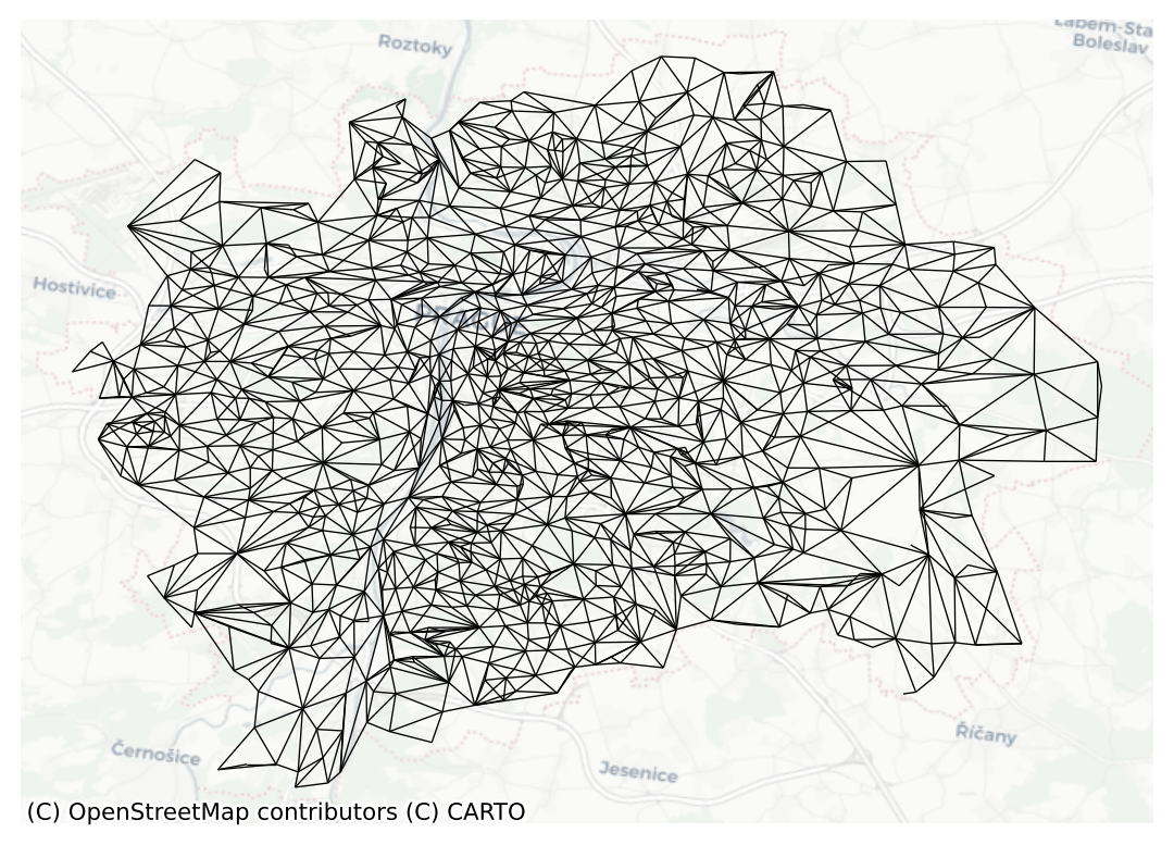

Once created, Graph objects can provide much information about the matrix beyond the basic attributes one would expect. You have direct access to the number of neighbours each observation has via the attribute cardinalities. For example, to find out how many neighbours observation E01006524 has:

queen.cardinalities['Albertov']

np.int64(9)

Since cardinalities is a Series, you can use all of the pandas functionality you know:

queen.cardinalities.head()

focal
Běchovice          3
Nová Dubeč         6
Benice             2
Březiněves         4
Dolní Černošice    4
Name: cardinalities, dtype: int64

You can easily compute the mean number of neighbours.

queen.cardinalities.mean()

np.float64(5.949632738719832)

Or learn about the maximum number of neighbours a single geometry has.

queen.cardinalities.max()

This also allows access to quick plotting, which comes in very handy in getting an overview of the size of neighbourhoods in general:

sns.displot(queen.cardinalities, bins=14, kde=True)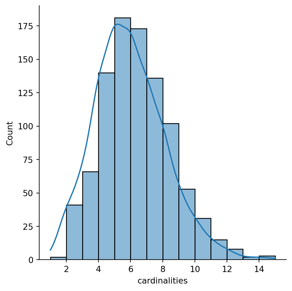

The figure above shows how most observations have around five neighbours, but there is some variation around it. The distribution also seems to follow nearly a symmetric form, where deviations from the average occur both in higher and lower values almost evenly, with a minor tail towards higher values.

Some additional information about the spatial relationships contained in the matrix is also easily available from a Graph object. You can ask about the number of observations (geometries) encoded in the graph:

queen.n

Or learn which geometries are isolates, the observations with no neighbours (think about islands).

1queen.isolates

1: In this case, this Series is empty since there are no isolates present.

Index([], dtype='object', name='focal')

A nice summary of these properties is available using the summary() method.

queen.summary()

Graph Summary Statistics
Number of nodes:	953
Number of edges:	5670
Number of connected components:	1
Number of isolates:	0
Number of non-zero edges:	5670
Percentage of non-zero edges:	0.62%
Number of asymmetries:	NA

Sum of weights and Traces
S0:	5670	GG:	5670
S1:	11340	G'G:	5670
S3:	153040	G'G + GG:	11340

Graph indexed by: ['Běchovice', 'Nová Dubeč', 'Benice', 'Březiněves', 'Doln...]

Spatial weight matrices can be explored visually in other ways. For example, you can pick an observation and visualise it in the context of its neighbourhood. The following plot does exactly that by zooming into the surroundings of ZSJ Albertov and displaying its polygon as well as those of its neighbours together with a relevant portion of the Graph:

m = prague.loc[queen["Albertov"].index].explore(color="#25b497")
prague.loc[["Albertov"]].explore(m=m, color="#fa94a5")
queen.explore(prague, m=m, focal="Albertov")

Make this Notebook Trusted to load map: File -> Trust Notebook

Rook

Rook contiguity is similar to and, in many ways, superseded by Queen contiguity. However, since it sometimes comes up in the literature, it is useful to know about it. The main idea is the same: two observations are neighbours if they share some of their boundary lines. However, in the Rook case, it is not enough to share only one point. It needs to be at least a segment of their boundary. In most applied cases, these differences usually boil down to how the geocoding was done, but in some cases, such as when you use raster data or grids, this approach can differ more substantively, and it thus makes more sense.

From a technical point of view, constructing a Rook matrix is very similar:

rook = graph.Graph.build_contiguity(prague, rook=True)
rook

<Graph of 953 nodes and 5210 nonzero edges indexed by
 ['Běchovice', 'Nová Dubeč', 'Benice', 'Březiněves', 'Dolní Černošice', ...]>

The output is of the same type as before, a Graph object that can be queried and used in very much the same way as any other one.

Bishop

In a similar sense, you may want to create Bishop contiguity - consider two geometries neighbouring if they share only one vertex. There’s no constructor for that but you can derive Bishop contiguity from Queen and Rook as Queen contains both shared vertex and shared edge relations. You can, therefore, subtract one from the other to get Bishop contiguity:

bishop = queen.difference(rook)
bishop

<Graph of 953 nodes and 460 nonzero edges indexed by
 ['Běchovice', 'Nová Dubeč', 'Benice', 'Březiněves', 'Dolní Černošice', ...]>

See the remaining edges:

ax = bishop.plot(prague, nodes=False, edge_kws={"linewidth": .5})
contextily.add_basemap(ax=ax, crs=prague.crs, source="CartoDB Positron")
ax.set_axis_off()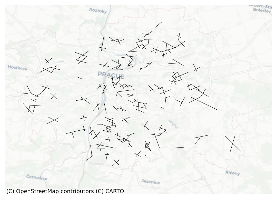

Bishop contiguity derived as a difference of Queen and Rook

Only a small fraction of Queen neighbours are not Rook neighbors at the same time (represented by the number of edges here), but there are some.

Distance

Distance-based matrices assign the weight to each pair of observations as a function of how far from each other they are. How this is translated into an actual weight varies across types and variants, but they all share that the ultimate reason why two observations are assigned some weight is due to the distance between them.

K-Nearest Neighbors

One approach to define weights is to take the distances between a given observation and the rest of the set, rank them, and consider as neighbours the \(k\) closest ones. That is exactly what the \(k\)-nearest neighbours (KNN) criterium does.

To calculate KNN weights, you can use a similar function as before and derive them from a GeoDataFrame:

1prague["centroid"] = prague.centroid
2prague = prague.set_geometry("centroid")
knn5 = graph.Graph.build_knn(prague, k=5)
knn5

1: Distance-based methods usually work only with points (for performance reasons). Create a centroid representation of each geometry.
2: Assign it as an active geometry column.

<Graph of 953 nodes and 4765 nonzero edges indexed by
 ['Běchovice', 'Nová Dubeč', 'Benice', 'Březiněves', 'Dolní Černošice', ...]>

See the resulting graph visually:

ax = knn5.plot(prague, nodes=False, edge_kws={"linewidth": .5})
contextily.add_basemap(ax=ax, crs=prague.crs, source="CartoDB Positron")
ax.set_axis_off()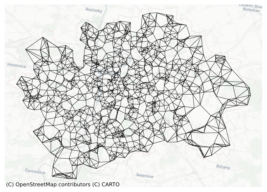

A graph representing 5 nearest neighbours

Note how you need to specify the number of nearest neighbours you want to consider with the argument k. Since it is a polygon GeoDataFrame that you are passing, you need to compute the centroids to derive distances between observations. Alternatively, you can provide the points in the form of an array, skipping this way the dependency of a file on disk:

pts = pd.DataFrame(
1    {"X": prague.geometry.x, "Y": prague.geometry.y}
2).values
knn5_from_pts = graph.Graph.build_knn(pts, k=5)

1: If your GeoSeries contains Point geometries, you can access their coordinates using GeoSeries.x and GeoSeries.y.
2: .values returns only an array of values without the pandas index. It is the underlying data structure coming from the numpy package. You will learn more about numpy in due course.

Distance band

Another approach to building distance-based spatial weights matrices is to draw a circle of certain radius and consider neighbour every observation that falls within the circle. The technique has two main variations: binary and continuous. In the former one, every neighbour is given a weight of one, while in the second one, the weights can be further tweaked by the distance to the observation of interest.

To compute binary distance matrices in PySAL, you can use the following command:

dist1kmB = graph.Graph.build_distance_band(prague, 1000)
dist1kmB

<Graph of 953 nodes and 6974 nonzero edges indexed by
 ['Běchovice', 'Nová Dubeč', 'Benice', 'Březiněves', 'Dolní Černošice', ...]>

This creates a binary matrix that considers neighbors of an observation every polygon whose centroid is closer than 1,000 metres (1 km) to the centroid of such observation. Check, for example, the neighbourhood of polygon Albertov:

dist1kmB['Albertov']

neighbor
Vodičkova                     1
Londýnská                     1
Štěpánský obvod-západ         1
Nad muzeem                    1
Folimanka-východ              1
Nuselské údolí                1
Vyšehrad                      1
Podskalí                      1
Zderaz                        1
U Čelakovského sadů           1
Štěpánský obvod-východ        1
Folimanka-západ               1
Nad Nuselským údolím          1
Na bělidle-nábřeží            1
Smíchovský pivovar-nábřeží    1
V Čelakovského sadech         1
Name: weight, dtype: int64

Note that the units in which you specify the distance directly depend on the CRS in which the spatial data are projected, and this has nothing to do with the weights building but it can affect it significantly. Recall how you can check the CRS of a GeoDataFrame:

prague.crs

<Projected CRS: EPSG:5514>
Name: S-JTSK / Krovak East North
Axis Info [cartesian]:
- X[east]: Easting (metre)
- Y[north]: Northing (metre)
Area of Use:
- name: Czechia; Slovakia.
- bounds: (12.09, 47.73, 22.56, 51.06)
Coordinate Operation:
- name: Krovak East North (Greenwich)
- method: Krovak (North Orientated)
Datum: System of the Unified Trigonometrical Cadastral Network
- Ellipsoid: Bessel 1841
- Prime Meridian: Greenwich

In this case, you can see the unit is expressed in metres (m). Hence you set the threshold to 1,000 for a circle of 1km radius. The whole graph looks like this:

ax = dist1kmB.plot(prague, nodes=False, edge_kws={"linewidth": .5})
contextily.add_basemap(ax=ax, crs=prague.crs, source="CartoDB Positron")
ax.set_axis_off()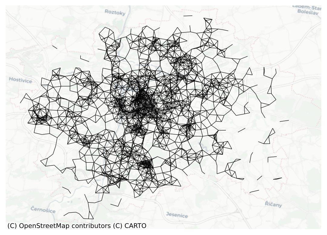

A graph representing distance band of 1 km.

Block weights

Block weights connect every observation in a dataset that belongs to the same category in a list provided ex-ante. Usually, this list will have some relation to geography and the location of the observations but, technically speaking, all one needs to create block weights is a list of memberships. In this class of weights, neighbouring observations, those in the same group, are assigned a weight of one, and the rest receive a weight of zero.

In this example, you will build a spatial weights matrix that connects every ZSJ with all the other ones in the same KU. See how the KU code is expressed for every ZSJ:

prague.head()

	NAZ_KU	n_people	geometry	centroid
NAZ_ZSJ
Běchovice	Běchovice	1563.0	MULTIPOLYGON (((-728432.898 -1045340.836, -728...	POINT (-728983.854 -1045559.217)
Nová Dubeč	Běchovice	662.0	MULTIPOLYGON (((-729878.896 -1045449.784, -729...	POINT (-730222.277 -1045630.462)
Benice	Benice	728.0	MULTIPOLYGON (((-730788.19 -1052695.343, -7307...	POINT (-730966.612 -1053057.39)
Březiněves	Březiněves	1808.0	MULTIPOLYGON (((-736983.473 -1034315.571, -737...	POINT (-737232.635 -1034903.671)
Dolní Černošice	Lipence	150.0	MULTIPOLYGON (((-748601.583 -1054231.394, -748...	POINT (-749780.041 -1055689.764)

To build a block spatial weights matrix that connects as neighbours all the ZSJ in the same KU, you only require the mapping of codes. Using PySAL, this is a one-line task:

block = graph.Graph.build_block_contiguity(prague['NAZ_KU'])
block

<Graph of 953 nodes and 11184 nonzero edges indexed by
 ['Běchovice', 'Nová Dubeč', 'Homole-U Čecha', 'Běchovice-jih', 'Běchovic...]>

If you query for the neighbors of observation by its name, it will work as usual:

block['Albertov']

neighbor
Petrský obvod                 1
Masarykovo nádraží            1
Jindřišský obvod              1
Vodičkova                     1
Vojtěšský obvod               1
Štěpánský obvod-západ         1
Podskalí                      1
Zderaz                        1
Autobusové nádraží Florenc    1
U Čelakovského sadů           1
Štěpánský obvod-východ        1
V Čelakovského sadech         1
Masarykovo nádraží-východ     1
Name: weight, dtype: int64

Notice the resulting blocks are clearly visible when you visualise the graph:

ax = block.plot(prague, nodes=False, edge_kws={"linewidth": .5})
contextily.add_basemap(ax=ax, crs=prague.crs, source="CartoDB Positron")
ax.set_axis_off()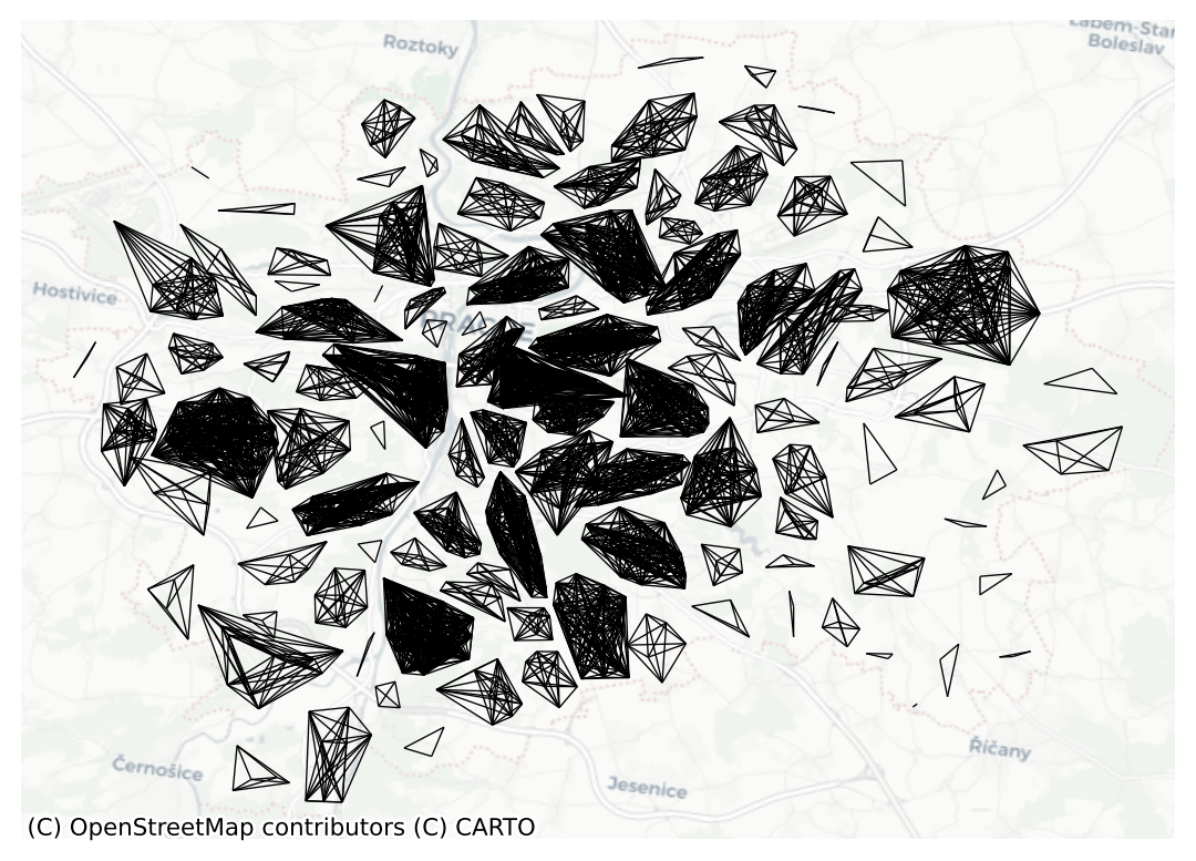

Weighted graphs

So far, all the graphs resulted in boolean weights. The two geometries either are neighbors or they are not. However, there are many situations where you want to give a different weight to each neighbor. For example, you may want to give a higher weight to those neighbors that are closer over those that are further away. Take the example of K-nearest neighbors.

knn5['Albertov']

neighbor
Štěpánský obvod-západ     1
Podskalí                  1
Zderaz                    1
Štěpánský obvod-východ    1
Folimanka-západ           1
Name: weight, dtype: int64

As you can see, all have the same weight - 1.

Kernel graphs

To make use of the actual distance, you can build a Kernel graph, where the distance between two points is passed to the kernel function deriving a weight from it.

1knn5_kernel = graph.Graph.build_kernel(prague, k=5)
knn5_kernel

1: As with KNN, kernel uses point-to-point distance. You can do kernel-weighted KNN by passing k.

<Graph of 953 nodes and 4765 nonzero edges indexed by
 ['Běchovice', 'Nová Dubeč', 'Benice', 'Březiněves', 'Dolní Černošice', ...]>

The default kernel is Gaussian but there’s a long list of built-in kernels and option to pass a custom function as well.

The resulting Graph has the same neighbors as the knn5 but the weight is derived from the distance between the points.

knn5_kernel['Albertov']

neighbor
Štěpánský obvod-západ     0.181761
Podskalí                  0.164128
Zderaz                    0.136754
Štěpánský obvod-východ    0.174166
Folimanka-západ           0.153312
Name: weight, dtype: float64

Distance-weighted distance band

An extension of the distance band weights above introduces further detail by assigning different weights to different neighbours within the radius circle based on how far they are from the observation of interest. For example, you could think of assigning the inverse of the distance between observations \(i\) and \(j\) as \(w_{ij}\). This can be computed with the following command:

dist1kmC = graph.Graph.build_distance_band(prague, 1000, binary=False)
dist1kmC

/home/runner/work/sds/sds/.pixi/envs/default/lib/python3.12/site-packages/libpysal/graph/base.py:812: RuntimeWarning: divide by zero encountered in power
  kernel=lambda distances, alpha: np.power(distances, alpha),

<Graph of 953 nodes and 6974 nonzero edges indexed by
 ['Běchovice', 'Nová Dubeč', 'Benice', 'Březiněves', 'Dolní Černošice', ...]>

In dist1kmC, every observation within the 1km circle is assigned a weight equal to the inverse distance between the two:

\[ w_{ij} = \dfrac{1}{d_{ij}} \]

This way, the further apart \(i\) and \(j\) are from each other, the smaller the weight \(w_{ij}\) will be.

Contrast the binary neighbourhood with the continuous one for Albertov:

dist1kmC['Albertov']

neighbor
Vodičkova                     0.001055
Londýnská                     0.001162
Štěpánský obvod-západ         0.002192
Nad muzeem                    0.001084
Folimanka-východ              0.001082
Nuselské údolí                0.001281
Vyšehrad                      0.001247
Podskalí                      0.001803
Zderaz                        0.001436
U Čelakovského sadů           0.001264
Štěpánský obvod-východ        0.002001
Folimanka-západ               0.001636
Nad Nuselským údolím          0.001183
Na bělidle-nábřeží            0.001158
Smíchovský pivovar-nábřeží    0.001000
V Čelakovského sadech         0.001121
Name: weight, dtype: float64

Following this logic of more detailed weights through distance, there is a temptation to take it further and consider everyone else in the dataset as a neighbor whose weight will then get modulated by the distance effect shown above. However, although conceptually correct, this approach is not always the most computationally or practical one. Because of the nature of spatial weights matrices, particularly because of the fact their size is \(N\) by \(N\), they can grow substantially large. A way to cope with this problem is by making sure they remain fairly sparse (with many zeros). Sparsity is typically ensured in the case of contiguity or KNN by construction but, with inverse distance, it needs to be imposed as, otherwise, the matrix could be potentially entirely dense (no zero values other than the diagonal). In practical terms, what is usually done is to impose a distance threshold beyond which no weight is assigned and interaction is assumed to be non-existent. Beyond being computationally feasible and scalable, results from this approach usually do not differ much from a fully “dense” one as the additional information that is included from further observations is almost ignored due to the small weight they receive. In this context, a commonly used threshold, although not always best, is that which makes every observation to have at least one neighbor.

Perimeter-weighted contiguity

Similarly, you can adapt contiguity graphs to derive weight from the proportion of the shared boundary between adjacent polygons.

prague = prague.set_geometry("geometry")
rook_by_perimeter = graph.Graph.build_contiguity(prague, by_perimeter=True)
rook_by_perimeter

<Graph of 953 nodes and 5210 nonzero edges indexed by
 ['Běchovice', 'Nová Dubeč', 'Benice', 'Březiněves', 'Dolní Černošice', ...]>

By default, the weight is the length of the shared boundary:

rook_by_perimeter['Albertov']

neighbor
Vodičkova                  357.250925
Vojtěšský obvod             88.091956
Štěpánský obvod-západ     1451.825524
Nuselské údolí              11.361159
Vyšehrad                   354.172040
Podskalí                   644.804410
Zderaz                     508.399865
Štěpánský obvod-východ     413.754231
Folimanka-západ            617.509605
Name: weight, dtype: float64

Computing threshold

Such a threshold can be calculated using the min_threshold_distance function from libpysal.weights module:

from libpysal import weights

min_thr = weights.min_threshold_distance(pts)
min_thr

np.float64(1920.0404365049942)

Which can then be used to calculate an inverse distance weights matrix:

min_dist = graph.Graph.build_distance_band(prague, min_thr, binary=False)

Standardizing `Graph` relationships

In the context of many spatial analysis techniques, a spatial weights matrix with raw values (e.g. ones and zeros for the binary case or lenghts for the perimeter-weighted contiguity) is not always the best-suiting one for analysis and some sort of transformation is required. This implies modifying each weight so they conform to certain rules. PySAL has transformations baked right into the Graph object, so it is possible to check the state of an object as well as to modify it.

Consider the original Queen weights for observation Albertov:

queen['Albertov']

neighbor
Vodičkova                 1
Vojtěšský obvod           1
Štěpánský obvod-západ     1
Nuselské údolí            1
Vyšehrad                  1
Podskalí                  1
Zderaz                    1
Štěpánský obvod-východ    1
Folimanka-západ           1
Name: weight, dtype: int64

Since it is contiguity, every neighbour gets one, the rest zero weight. You can check if the object queen has been transformed or not by calling the property .transformation:

queen.transformation

'O'

where "O" stands for “original”, so no transformations have been applied yet. If you want to apply a row-based transformation so every row of the matrix sums up to one, you use the .transform() method as follows:

1row_wise_queen = queen.transform("R")

1: .transform() returns a new Graph with transformed weights. "R" stands for row-wise transformation.

Now you can check the weights of the same observation as above and find they have been modified:

row_wise_queen['Albertov']

neighbor
Vodičkova                 0.111111
Vojtěšský obvod           0.111111
Štěpánský obvod-západ     0.111111
Nuselské údolí            0.111111
Vyšehrad                  0.111111
Podskalí                  0.111111
Zderaz                    0.111111
Štěpánský obvod-východ    0.111111
Folimanka-západ           0.111111
Name: weight, dtype: float64

The sum of weights for all the neighbours is one:

row_wise_queen['Albertov'].sum()

np.float64(1.0)

PySAL currently supports the following transformations:

O: original, returning the object to the initial state.
B: binary, with every neighbour having assigned a weight of one.
R: row, with all the neighbours of a given observation adding up to one.
V: variance stabilising, with the sum of all the weights being constrained to the number of observations.
D: double, with all the weights across all observations adding up to one.

The same can be done with non-binary weights. Given the example of perimeter-weighted Rook contiguity created above, you can transform the lengths of shared boundaries to a row-normalised value.

rook_by_perimeter['Albertov']

neighbor
Vodičkova                  357.250925
Vojtěšský obvod             88.091956
Štěpánský obvod-západ     1451.825524
Nuselské údolí              11.361159
Vyšehrad                   354.172040
Podskalí                   644.804410
Zderaz                     508.399865
Štěpánský obvod-východ     413.754231
Folimanka-západ            617.509605
Name: weight, dtype: float64

Transform the weights:

rook_by_perimeter_row = rook_by_perimeter.transform("R")
rook_by_perimeter_row['Albertov']

neighbor
Vodičkova                 0.080332
Vojtěšský obvod           0.019809
Štěpánský obvod-západ     0.326461
Nuselské údolí            0.002555
Vyšehrad                  0.079640
Podskalí                  0.144992
Zderaz                    0.114320
Štěpánský obvod-východ    0.093038
Folimanka-západ           0.138855
Name: weight, dtype: float64

This may be necessary for certain statistical operations assuming a sum of weights in a row equals to 1.

Reading and Writing spatial weights in `PySAL`

Sometimes, suppose a dataset is very detailed or large. In that case, it can be costly to build the spatial weights matrix of a given geography, and, despite the optimisations in the PySAL code, the computation time can quickly grow out of hand. In these contexts, it is useful not to have to rebuild a matrix from scratch every time you need to re-run the analysis. A useful solution, in this case, is to build the matrix once and save it to a file where it can be reloaded at a later stage if needed.

PySAL has a way to efficiently write any kind of Graph object into a file using the method .to_parquet(). This will serialise the underlying adjacency table into an Apache Parquet file format that is very fast to read and write and can be compressed to a small size.

queen.to_parquet("queen.parquet")

You can then read such a file back to the Graph from using graph.read_parquet() function:

queen_2 = graph.read_parquet("queen.parquet")

Interoperabilty with other tools

Weights saved as a Parquet file are efficient if PySAL is the only tool you want to use to read and write them. If you want to save them to other file formats like GAL or GWT that are readable by tools like GeoDa, you can save graphs to interoperable GAL (binary) or GWT (non-binary) formats using:

queen.to_gal("queen.gal")

queen.to_gwt("queen.gwt")

Similarly, you can read such files with graph.read_gal() and graph.read_gwt().

Using graph to aggregate variables

A typical use of a graph is a description of the distribution of values within the neighborhood of each geometry. This can be done either solely based on the neighborhood definition, ignoring the actual weight, or as a weighted operation.

Describe

The first option is implemented within the describe() method, which returns a statistical description of distribution of a given variable within each neighborhood.

For this illustration, you will use the area of each polygon as the variable of interest. And to make things a bit nicer later on, you will keep the log of the area instead of the raw measurement. Hence, let’s create a column for it:

1prague = prague.set_geometry("geometry")
2prague["area"] = np.log(prague.area)

1: Remember to set active geometry back to polygons before computing area.
2: np.log is a function from the numpy package that computes the natural logarithm of an array of values (elementwise).

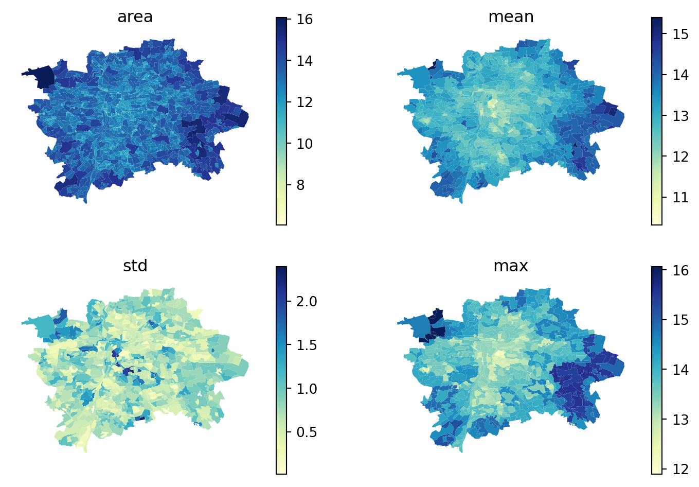
area_description = queen.describe(
    prague["area"],
    statistics=["mean", "median", "min", "max", "std"],
)
area_description.head()

	mean	median	min	max	std
focal
Běchovice	13.842025	13.807607	12.884636	14.833831	0.975053
Nová Dubeč	14.064429	13.663940	13.314663	15.544656	0.916046
Benice	13.834280	13.834280	13.319198	14.349361	0.728435
Březiněves	14.193854	14.174226	14.118746	14.308217	0.085135
Dolní Černošice	14.102750	14.196712	13.474719	14.542857	0.526936

The table can be directly assigned to the prague DataFrame, if needed.

prague = prague.join(area_description)
prague.head()

	NAZ_KU	n_people	geometry	centroid	area	mean	median	min	max	std
NAZ_ZSJ
Běchovice	Běchovice	1563.0	MULTIPOLYGON (((-728432.898 -1045340.836, -728...	POINT (-728983.854 -1045559.217)	13.314663	13.842025	13.807607	12.884636	14.833831	0.975053
Nová Dubeč	Běchovice	662.0	MULTIPOLYGON (((-729878.896 -1045449.784, -729...	POINT (-730222.277 -1045630.462)	12.884636	14.064429	13.663940	13.314663	15.544656	0.916046
Benice	Benice	728.0	MULTIPOLYGON (((-730788.19 -1052695.343, -7307...	POINT (-730966.612 -1053057.39)	13.037903	13.834280	13.834280	13.319198	14.349361	0.728435
Březiněves	Březiněves	1808.0	MULTIPOLYGON (((-736983.473 -1034315.571, -737...	POINT (-737232.635 -1034903.671)	13.372632	14.193854	14.174226	14.118746	14.308217	0.085135
Dolní Černošice	Lipence	150.0	MULTIPOLYGON (((-748601.583 -1054231.394, -748...	POINT (-749780.041 -1055689.764)	15.172999	14.102750	14.196712	13.474719	14.542857	0.526936

Compare a subset visually on a map. You can create a subplot with 4 axes and loop over the selected columns to do that efficiently.

1columns = ["area", "mean", "std", "max"]

2fig, axs = plt.subplots(2, 2, figsize=(9, 6))
3axs = axs.flatten()
4for column, ax in zip(columns, axs):
5    prague.plot(column, ax=ax, legend=True, cmap="YlGnBu")
6    ax.set_axis_off()
7    ax.set_title(column)

1: Specify a list of columns to be plotted.
2: Create a figure with 4 subplots in a 2x2 grid, sized 9x6 inches.
3: Flatten the axis for easier iteration.
4: Make a for loop over two arrays at the same time zipped together.
5: Make the map, show its legend and assign a custom colormap.
6: Disable axis boundary plotting.
7: Set title of each subplot.

Log of area and its derivatives based on Queen contiguity

Spatial Lag

If you need to use the weight, you are looking for the so-called spatial lag. The spatial lag of a given variable is the product of a spatial weight matrix and the variable itself:

\[ Y_{sl} = W Y \]

where \(Y\) is a Nx1 vector with the values of the variable. Recall that the product of a matrix and a vector equals the sum of a row by column element multiplication for the resulting value of a given row. In terms of the spatial lag:

\[ y_{sl-i} = \displaystyle \sum_j w_{ij} y_j \]

If you are using row-standardized weights, \(w_{ij}\) becomes a proportion between zero and one, and \(y_{sl-i}\) can be seen as the mean value of \(Y\) in the neighborhood of \(i\), the same you would get with describe().

The spatial lag is a key element of many spatial analysis techniques, as you will see later on and, as such, it is fully supported in PySAL. To compute the spatial lag of a given variable, area, for example:

1queen_lag = row_wise_queen.lag(prague["area"])
2queen_lag[:5]

1: Compute spatial lag of area using row-wised standardised weights to get mean values. If you used binary weights, the resulting spatial lag would equal to sum of values.
2: Print the first five elements

array([13.84202483, 14.06442931, 13.83427974, 14.19385395, 14.10275008])

Line 1 contains the actual computation, which is highly optimised in PySAL. Note that, despite passing in a pd.Series object, the output is a numpy array. This however, can be added directly to the table prague:

prague['area_lag'] = queen_lag

Categorical lag

If you have categorical data, you can use the categorical lag, which returns the most common category within the neighbors. You can try with the KU name.

categorical_lag = row_wise_queen.lag(prague["NAZ_KU"], ties="tryself")
categorical_lag[:5]

array(['Nové Město', 'Kyje', 'Smíchov', 'Krč', 'Smíchov'], dtype=object)

Note that when there is a tie, i.e., no category is the most common, lag() will raise an error by default. You can let it resolve ties either by including the value from the focal observation to break the tie or by picking the one randomly (ties="random").

Acknowledgements

This section is derived from A Course on Geographic Data Science by Arribas-Bel (2019), licensed under CC-BY-SA 4.0. The code was updated to use the new libpysal.graph module instead of libpysal.weights. The text was slightly adapted to accommodate a different dataset and the module change.

References

Arribas-Bel, Dani. 2019. “A Course on Geographic Data Science.” The Journal of Open Source Education 2 (14). https://doi.org/10.21105/jose.00042.

Data

Building spatial weights in PySAL

Contiguity

Queen

Rook

Bishop

Distance

K-Nearest Neighbors

Distance band

Block weights

Weighted graphs

Kernel graphs

Distance-weighted distance band

Perimeter-weighted contiguity

Standardizing Graph relationships

Reading and Writing spatial weights in PySAL

Using graph to aggregate variables

Describe

Spatial Lag

Categorical lag

Acknowledgements

References

Building spatial weights in `PySAL`

Standardizing `Graph` relationships

Reading and Writing spatial weights in `PySAL`