Regression and geography

When trying to determine the effect of some (independent) variables on the outcome of phenomena (dependent variable), you often use regression to model such an outcome and understand the influence each of the variables has in the model. With spatial regression, it is the same. You just need to use the spatial dimension in a mindful way.

This session provides an introduction to ways of incorporating space into regression models, from spatial variables in standard linear regression to geographically weighted regression.

import esda
import geopandas as gpd
import matplotlib.pyplot as plt
import mgwr
import numpy as np
import pandas as pd
import seaborn as sns
import statsmodels.formula.api as sm
from libpysal import graph

Data

You will work with the same data you already used in the session on spatial autocorrelation - the results of the second round of the presidential elections in Czechia in 2023, between Petr Pavel and Andrej Babiš, on a level of municipalities. You can read the election data directly from the original location.

elections = gpd.read_file(
    "https://martinfleischmann.net/sds/autocorrelation/data/cz_elections_2023.gpkg"
)
elections = elections.set_index("name")
elections.head()

	nationalCode	PetrPavel	AndrejBabis	sourceOfName	geometry
name
Želechovice nad Dřevnicí	500011	61.73	38.26	Český úřad zeměměřický a katastrální	MULTIPOLYGON (((-518835.63 -1170505.52, -51790...
Petrov nad Desnou	500020	49.07	50.92	Český úřad zeměměřický a katastrální	MULTIPOLYGON (((-559207.18 -1075123.25, -55624...
Libhošť	500046	47.78	52.21	Český úřad zeměměřický a katastrální	MULTIPOLYGON (((-486502.29 -1123694.06, -48717...
Krhová	500062	58.79	41.20	Český úřad zeměměřický a katastrální	MULTIPOLYGON (((-494514.83 -1136457.23, -49539...
Poličná	500071	58.20	41.79	Český úřad zeměměřický a katastrální	MULTIPOLYGON (((-499678.51 -1143457.52, -49799...

Alternative

Instead of reading the file directly off the web, it is possible to download it manually, store it on your computer, and read it locally. To do that, you can follow these steps:

Download the file by right-clicking on this link and saving the file
Place the file in the same folder as the notebook where you intend to read it
Replace the code in the cell above with:

elections = gpd.read_file(
    "cz_elections_2023.gpkg",
)

The election results give you the dependent variable - you will look at the percentage of votes Petr Pavel, the winner, received. From the map of the results and the analysis you did when exploring spatial autocorrelation you already know that there are some significant spatial patterns. Let’s look whether these patterns correspond to the composition of education levels within each municipality.

You can use the data from the Czech Statistical Office reflecting the situation during the Census 2021. The original table has been preprocessed and is available as a CSV.

education = pd.read_csv(
    "https://martinfleischmann.net/sds/regression/data/education.csv"
)
education.head()

	uzemi_kod	without_education	undetermined	incomplete_primary_education	lower_secondary_and_secondary_education	further_education	post_maturita_studies	bachelors_degree	doctoral_degree	masters_degree	higher_vocational_education	higher_vocational_education_in_a_conservatory	primary_education	complete_secondary_vocational_education	complete_secondary_general_education	okres
0	500011	0.570704	3.741281	1.141408	34.242232	1.775523	0.507292	2.853519	0.634115	12.935954	1.395054	0.126823	11.350666	17.945466	10.779962	Zlín
1	500020	0.885827	3.346457	1.968504	40.157480	2.066929	0.885827	1.771654	0.492126	6.299213	1.574803	0.000000	15.059055	16.338583	9.153543	Šumperk
2	500046	0.359195	3.232759	0.790230	39.152299	2.514368	0.790230	3.520115	0.215517	10.632184	1.364943	0.143678	9.770115	15.301724	12.212644	Nový Jičín
3	500062	0.238237	3.573556	1.072067	32.757594	2.084574	1.131626	3.037522	0.178678	13.281715	0.714711	0.119119	11.316260	18.701608	11.792734	Vsetín
4	500071	0.412939	2.890571	1.238816	34.067447	1.720578	0.757054	3.028217	0.137646	11.080523	0.894701	0.000000	9.772884	20.027529	13.971094	Vsetín

Alternative

Instead of reading the file directly off the web, it is possible to download it manually, store it on your computer, and read it locally. To do that, you can follow these steps:

Download the file by right-clicking on this link and saving the file
Place the file in the same folder as the notebook where you intend to read it
Replace the code in the cell above with:

education = pd.read_csv(
    "education.csv",
)

The first thing you need to do is to merge the two tables, to have both dependent and independent variables together. The municipality code in the elections table is in the "nationalCode" column, while in the education table in the "uzemi_kod" column.

elections_data = elections.merge(education, left_on="nationalCode", right_on="uzemi_kod")
elections_data.head()

	nationalCode	PetrPavel	AndrejBabis	sourceOfName	geometry	uzemi_kod	without_education	undetermined	incomplete_primary_education	lower_secondary_and_secondary_education	...	post_maturita_studies	bachelors_degree	doctoral_degree	masters_degree	higher_vocational_education	higher_vocational_education_in_a_conservatory	primary_education	complete_secondary_vocational_education	complete_secondary_general_education	okres
0	500011	61.73	38.26	Český úřad zeměměřický a katastrální	MULTIPOLYGON (((-518835.63 -1170505.52, -51790...	500011	0.570704	3.741281	1.141408	34.242232	...	0.507292	2.853519	0.634115	12.935954	1.395054	0.126823	11.350666	17.945466	10.779962	Zlín
1	500020	49.07	50.92	Český úřad zeměměřický a katastrální	MULTIPOLYGON (((-559207.18 -1075123.25, -55624...	500020	0.885827	3.346457	1.968504	40.157480	...	0.885827	1.771654	0.492126	6.299213	1.574803	0.000000	15.059055	16.338583	9.153543	Šumperk
2	500046	47.78	52.21	Český úřad zeměměřický a katastrální	MULTIPOLYGON (((-486502.29 -1123694.06, -48717...	500046	0.359195	3.232759	0.790230	39.152299	...	0.790230	3.520115	0.215517	10.632184	1.364943	0.143678	9.770115	15.301724	12.212644	Nový Jičín
3	500062	58.79	41.20	Český úřad zeměměřický a katastrální	MULTIPOLYGON (((-494514.83 -1136457.23, -49539...	500062	0.238237	3.573556	1.072067	32.757594	...	1.131626	3.037522	0.178678	13.281715	0.714711	0.119119	11.316260	18.701608	11.792734	Vsetín
4	500071	58.20	41.79	Český úřad zeměměřický a katastrální	MULTIPOLYGON (((-499678.51 -1143457.52, -49799...	500071	0.412939	2.890571	1.238816	34.067447	...	0.757054	3.028217	0.137646	11.080523	0.894701	0.000000	9.772884	20.027529	13.971094	Vsetín

5 rows × 21 columns

That is all sorted and ready to be used in a regression.

Non-spatial linear regression

Before jumping into spatial regression, let’s start with the standard linear regression. A useful start is to explore the data using an ordinary least squares (OLS) linear regression model.

OLS model

While this course is not formula-heavy, in this case, it is useful to use the formula to explain the logic of the algorithm. The OLS tries to model the dependent variable \(y\) as the linear combination of independent variables \(x_1, x_2, ... x_n\):

\[y_{i}=\alpha+\beta _{1}\ x_{i1}+\beta _{2}\ x_{i2}+\cdots +\beta _{p}\ x_{ip}+\varepsilon _{i}\]

where \(\epsilon_{i}\) represents unobserved random variables and \(\alpha\) represents an intercept - a constant. You know the \(y_i\), all of the \(x_i\) and try to estimate the coefficients. In Python, you can run linear regression using implementations from more than one package (e.g., statsmodels, scikit-learn, spreg). This course covers statsmodels approach as it has a nice API to work with.

First, you need a list of names of independent variables. That is equal to column names without a few of the columns that represent other data.

independent_names = education.columns.drop(["uzemi_kod", "okres"])
independent_names

Index(['without_education', 'undetermined', 'incomplete_primary_education',
       'lower_secondary_and_secondary_education', 'further_education',
       'post_maturita_studies', 'bachelors_degree', 'doctoral_degree',
       'masters_degree', 'higher_vocational_education',
       'higher_vocational_education_in_a_conservatory', 'primary_education',
       'complete_secondary_vocational_education',
       'complete_secondary_general_education'],
      dtype='object')

statsmodels (above imported as sm) offers an intuitive formula API to define the linear regression.

1formula = f"PetrPavel ~ {' + '.join(independent_names)}"
formula

1: In the formula, specify the dependent variable ("PetrPavel") as a function of ("~") independent variables ("undetermined + incomplete_primary_education + ...").

'PetrPavel ~ without_education + undetermined + incomplete_primary_education + lower_secondary_and_secondary_education + further_education + post_maturita_studies + bachelors_degree + doctoral_degree + masters_degree + higher_vocational_education + higher_vocational_education_in_a_conservatory + primary_education + complete_secondary_vocational_education + complete_secondary_general_education'

With the formula ready, you can fit the model and estimate all betas and \(\varepsilon\).

ols = sm.ols(formula, data=elections_data).fit()

The ols object offers a handy summary() function providing most of the results from the fitting in one place.

ols.summary()

OLS Regression Results
Dep. Variable:	PetrPavel	R-squared:	0.423
Model:	OLS	Adj. R-squared:	0.422
Method:	Least Squares	F-statistic:	352.6
Date:	Mon, 21 Apr 2025	Prob (F-statistic):	0.00
Time:	11:51:03	Log-Likelihood:	-22397.
No. Observations:	6254	AIC:	4.482e+04
Df Residuals:	6240	BIC:	4.492e+04
Df Model:	13
Covariance Type:	nonrobust

	coef	std err	t	P>\|t\|	[0.025	0.975]
Intercept	0.1283	0.006	19.748	0.000	0.116	0.141
without_education	0.3621	0.093	3.914	0.000	0.181	0.543
undetermined	0.1879	0.041	4.542	0.000	0.107	0.269
incomplete_primary_education	-0.0881	0.119	-0.737	0.461	-0.322	0.146
lower_secondary_and_secondary_education	0.2890	0.013	21.435	0.000	0.263	0.315
further_education	0.9665	0.116	8.312	0.000	0.739	1.194
post_maturita_studies	1.3528	0.204	6.635	0.000	0.953	1.752
bachelors_degree	1.1634	0.092	12.581	0.000	0.982	1.345
doctoral_degree	1.2223	0.220	5.550	0.000	0.791	1.654
masters_degree	1.1231	0.036	31.201	0.000	1.053	1.194
higher_vocational_education	1.7312	0.132	13.124	0.000	1.473	1.990
higher_vocational_education_in_a_conservatory	2.7664	0.577	4.796	0.000	1.636	3.897
primary_education	0.0723	0.033	2.213	0.027	0.008	0.136
complete_secondary_vocational_education	0.8683	0.032	27.316	0.000	0.806	0.931
complete_secondary_general_education	0.8121	0.038	21.247	0.000	0.737	0.887

Omnibus:	130.315	Durbin-Watson:	1.680
Prob(Omnibus):	0.000	Jarque-Bera (JB):	215.929
Skew:	0.189	Prob(JB):	1.29e-47
Kurtosis:	3.828	Cond. No.	6.06e+17

Notes:
[1] Standard Errors assume that the covariance matrix of the errors is correctly specified.
[2] The smallest eigenvalue is 3.61e-29. This might indicate that there are
strong multicollinearity problems or that the design matrix is singular.

It is clear that education composition has a significant effect on the outcome of the elections but can explain only about 42% of its variance (adjusted \(R^2\) is 0.422). A higher amount of residents with only primary education tends to lower Pavel’s gain while a higher amount of university degrees tends to increase the number of votes he received. That is nothing unexpected. However, let’s make use of geography and unpack these results a bit.

Spatial exploration of the model (hidden structures)

Start with the visualisation of the prediction the OLS model produces using the coefficients shown above.

1predicted = ols.predict(elections_data)
predicted.head()

1: Use the predict() method with the original data to get the prediction using the model.

0    59.782801
1    50.879659
2    58.582439
3    60.674179
4    60.372217
dtype: float64

Make a plot comparing the prediction with the actual results.

1f, axs = plt.subplots(2, 1, figsize=(7, 8))
2elections_data.plot(
    predicted, legend=True, cmap="coolwarm", vmin=0, vmax=100, ax=axs[0]
)
3elections_data.plot(
    "PetrPavel", legend=True, cmap="coolwarm", vmin=0, vmax=100, ax=axs[1]
)
4axs[0].set_title("OLS prediction")
axs[1].set_title("Actual results")

5axs[0].set_axis_off()
axs[1].set_axis_off()

1: Create a subplot with two axes.
2: Plot the predicted data on the elections_data geometry.
3: Plot the original results.
4: Set titles for axes in the subplot.
5: Remove axes borders.

The general patterns are captured but there are some areas of the country which seem to be quite off. The actual error between prediction and the dependent variable is captured as residuals, which are directly available in ols as ols.resid attribute. Let’s plot to get a better comparison.

1elections_data["residual"] = ols.resid
2max_residual = ols.resid.abs().max()
3ax = elections_data.plot(
    "residual", legend=True, cmap="RdBu", vmin=-max_residual, vmax=max_residual
)
ax.set_axis_off()

1: Assign residuals as a column. This is not needed for the plot but it will be useful later.
2: Identify the maximum residual value based on absolute value to specify vmin and vmax values of the colormap.
3: Plot the data using diverging colormap centred around 0.

All of the municipalities in blue (residual above 0) have reported higher gains for Petr Pavel than the model assumes based on education structure, while all in red reported lower gains than what is expected. However, as data scientists, we have better tools to analyse the spatial structure of residuals than eyeballing it. Let’s recall the session on spatial autocorrelation again and figure out the spatial clusters of residuals.

First, create a contiguity graph and row-normalise it.

contiguity_r = graph.Graph.build_contiguity(elections_data).transform("r")

Then you can generate a Moran plot of residuals. For that, you will need the lag of residuals.

elections_data["residual_lag"] = contiguity_r.lag(elections_data["residual"])

And then you can use the code from the earlier session to generate a Moran scatterplot using seaborn.

f, ax = plt.subplots(1, figsize=(6, 6))
sns.regplot(
    x="residual",
    y="residual_lag",
    data=elections_data,
    marker=".",
    scatter_kws={"alpha": 0.2},
    line_kws=dict(color="lightcoral")
)
plt.axvline(0, c="black", alpha=0.5)
plt.axhline(0, c="black", alpha=0.5);

That looks like a pretty strong relationship. Use the local version of Moran’s statistic to find out the clusters.

1lisa = esda.Moran_Local(elections_data['residual'], contiguity_r)

1: Use Moran_Local function from esda.

Let’s visualise the results.

lisa.explore(elections_data, prefer_canvas=True, tiles="CartoDB Positron")

Make this Notebook Trusted to load map: File -> Trust Notebook

LISA clusters

The outcome of LISA shows large clusters of both overpredicted (High-High) and underpredicted (Low-Low) areas. The underpredicted are mostly in central Bohemia around Prague and in the mountains near the borders, where the ski resorts are. Putting aside the central areas for a bit, the explanation of underprediction in mountains is relatively straightforward. The education data are linked to the residents of each municipality. The people who voted in a municipality do not necessarily need to match with residents. It is known that more affluent population groups, who are more likely to go to a ski resort, voted overwhelmingly for Pavel. And since the elections were in winter, a lot of them likely voted in ski resorts, affecting the outcome of the model.

The overpredicted areas, on the other hand, are known for higher levels of deprivation, which may have played a role in the results. What is clear, is that geography plays a huge role in the modelling of the elections.

Spatial heterogeneity

Not all areas behave equally, it seems that some systematically vote for Pavel more than for Babiš while others vote for him less. You need to account for this when building a regression model. One way is by capturing spatial heterogeneity. It implicitly assumes that the outcome of the model spatially varies. You can expect \(\alpha\) to vary across space, or individual values of \(\beta\). Spatial fixed effects capture the former.

Spatial fixed effects

You need to find a way to let \(\alpha\) change across space. One option is through the proxy variable capturing higher-level geography. You have information about okres (the closest translation to English would probably be district or county) each municipality belongs to. Let’s start by checking if that could be useful by visualising residuals within each. While you can use the box plot directly, it may be better to sort the values by median residuals, so let’s complicate the code a bit.

1medians = (
    elections_data.groupby("okres")
    .residual.median()
    .to_frame("okres_residual")
)
f, ax = plt.subplots(figsize=(16, 6))
2sns.boxplot(
3    data=elections_data.merge(
        medians, how="left", left_on="okres", right_index=True
4    ).sort_values("okres_residual"),
5    x="okres",
6    y="residual",
)
7_ = plt.xticks(rotation=90)

1: Get median residual value per okres using groupby and convert the resulting Series to DataFrame to be able to merge it with the original data.
2: Create a box plot and pass the data.
3: The data is the elections_data table merged with the medians that are after merge stored as the "okres_residual" column.
4: Sort by the "okres_residual" column.
5: The x value should represent each okres.
6: The y value should represent residuals.
7: Rotate x tick labels by 90 degrees for readability.

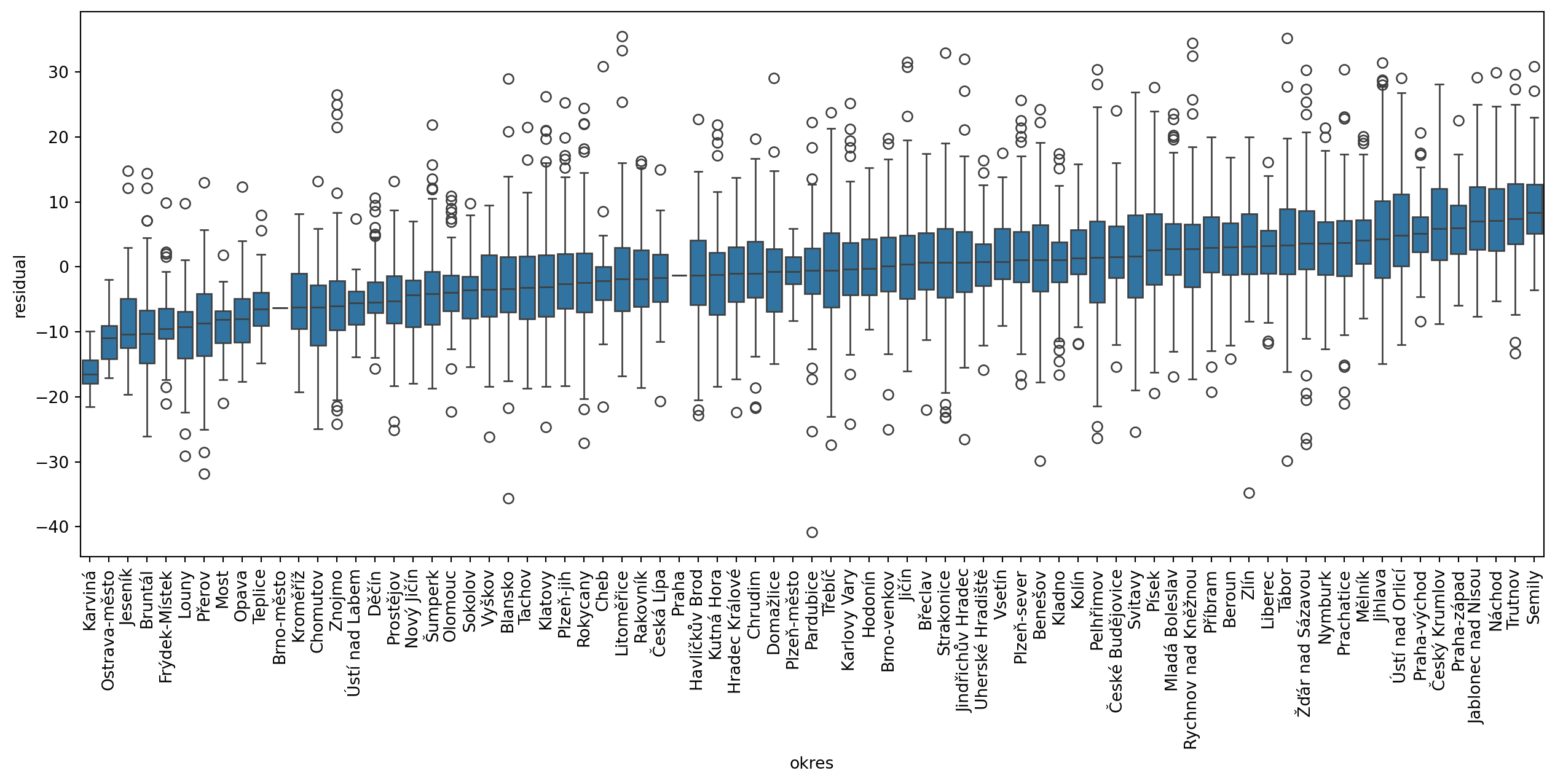
There are clear differences among these geographies, with a gradient between median -16.5 and 8.3. In a model that does not show spatial heterogeneity across higher-level geographies like these, all medians would be close to zero. This is positive information as it indicates, that we can encode these geographies in the model as a spatial proxy. Using statsmodels, you can adapt the equation and include "okres" as a dummy variable.

1formula_fe = f"PetrPavel ~ {' + '.join(independent_names)} + okres - 1"
2ols_fe = sm.ols(formula_fe, data=elections_data).fit()

1: Add + okres - 1, where - 1 means that you’re fitting a model without an intercept. Since you are now including a categorical variable okres, that will be converted to a dummy one, statsmodels would otherwise drop the first level (okres) to use as a reference represented by the intercept. The resulting coefficients would then reflect the difference between the intercept and the value for each okres. By omitting the intercept, the coefficient can be directly interpreted as \(\alpha\).
2: Fit the OLS model using the new formula.

Since every unique value in the "okres" column is now treated as a unique variable the summary is a bit longer than before.

ols_fe.summary()

OLS Regression Results
Dep. Variable:	PetrPavel	R-squared:	0.571
Model:	OLS	Adj. R-squared:	0.565
Method:	Least Squares	F-statistic:	92.21
Date:	Mon, 21 Apr 2025	Prob (F-statistic):	0.00
Time:	11:51:20	Log-Likelihood:	-21472.
No. Observations:	6254	AIC:	4.312e+04
Df Residuals:	6164	BIC:	4.373e+04
Df Model:	89
Covariance Type:	nonrobust

	coef	std err	t	P>\|t\|	[0.025	0.975]
okres[Benešov]	2.5515	0.725	3.520	0.000	1.131	3.972
okres[Beroun]	4.3517	0.834	5.219	0.000	2.717	5.986
okres[Blansko]	-1.0237	0.723	-1.416	0.157	-2.441	0.393
okres[Brno-město]	-3.6810	7.473	-0.493	0.622	-18.331	10.968
okres[Brno-venkov]	1.9413	0.593	3.276	0.001	0.779	3.103
okres[Bruntál]	-10.4042	0.938	-11.094	0.000	-12.243	-8.566
okres[Břeclav]	1.2036	0.957	1.258	0.209	-0.673	3.080
okres[Cheb]	-2.6902	1.204	-2.234	0.026	-5.051	-0.330
okres[Chomutov]	-7.3448	1.145	-6.417	0.000	-9.589	-5.101
okres[Chrudim]	0.5374	0.744	0.722	0.470	-0.921	1.996
okres[Domažlice]	-0.5435	0.880	-0.618	0.537	-2.268	1.181
okres[Děčín]	-4.6916	1.061	-4.424	0.000	-6.771	-2.613
okres[Frýdek-Místek]	-7.5664	0.907	-8.345	0.000	-9.344	-5.789
okres[Havlíčkův Brod]	0.3325	0.717	0.464	0.643	-1.073	1.738
okres[Hodonín]	0.5302	0.845	0.628	0.530	-1.126	2.187
okres[Hradec Králové]	-0.0895	0.755	-0.119	0.906	-1.570	1.391
okres[Jablonec nad Nisou]	9.3049	1.275	7.300	0.000	6.806	11.804
okres[Jeseník]	-7.5762	1.537	-4.930	0.000	-10.589	-4.564
okres[Jihlava]	5.8273	0.701	8.311	0.000	4.453	7.202
okres[Jindřichův Hradec]	2.4094	0.749	3.218	0.001	0.942	3.877
okres[Jičín]	1.7354	0.735	2.362	0.018	0.295	3.176
okres[Karlovy Vary]	0.3530	1.027	0.344	0.731	-1.661	2.367
okres[Karviná]	-15.8537	1.819	-8.716	0.000	-19.419	-12.288
okres[Kladno]	1.9768	0.771	2.564	0.010	0.465	3.488
okres[Klatovy]	-1.2087	0.791	-1.528	0.126	-2.759	0.342
okres[Kolín]	2.9124	0.809	3.602	0.000	1.327	4.498
okres[Kroměříž]	-4.4764	0.859	-5.212	0.000	-6.160	-2.793
okres[Kutná Hora]	-0.5966	0.819	-0.728	0.466	-2.202	1.009
okres[Liberec]	2.7545	0.988	2.788	0.005	0.817	4.691
okres[Litoměřice]	-0.6300	0.751	-0.838	0.402	-2.103	0.843
okres[Louny]	-10.6715	0.916	-11.655	0.000	-12.466	-8.877
okres[Mladá Boleslav]	4.5057	0.708	6.361	0.000	3.117	5.894
okres[Most]	-9.2808	1.479	-6.275	0.000	-12.180	-6.381
okres[Mělník]	5.0893	0.917	5.548	0.000	3.291	6.888
okres[Nový Jičín]	-4.1418	1.032	-4.013	0.000	-6.165	-2.119
okres[Nymburk]	3.9077	0.825	4.734	0.000	2.290	5.526
okres[Náchod]	8.7053	0.866	10.055	0.000	7.008	10.403
okres[Olomouc]	-2.8127	0.779	-3.613	0.000	-4.339	-1.286
okres[Opava]	-7.1956	0.871	-8.261	0.000	-8.903	-5.488
okres[Ostrava-město]	-9.5847	2.088	-4.590	0.000	-13.679	-5.491
okres[Pardubice]	0.5159	0.729	0.708	0.479	-0.914	1.945
okres[Pelhřimov]	2.2828	0.709	3.221	0.001	0.894	3.672
okres[Plzeň-jih]	-1.2318	0.772	-1.595	0.111	-2.745	0.282
okres[Plzeň-město]	1.2374	1.939	0.638	0.523	-2.565	5.039
okres[Plzeň-sever]	2.3828	0.775	3.074	0.002	0.863	3.902
okres[Prachatice]	3.5268	0.943	3.739	0.000	1.678	5.376
okres[Praha]	1.5703	7.475	0.210	0.834	-13.082	16.223
okres[Praha-východ]	7.3812	0.764	9.657	0.000	5.883	8.880
okres[Praha-západ]	8.0313	0.914	8.791	0.000	6.240	9.822
okres[Prostějov]	-4.1691	0.780	-5.345	0.000	-5.698	-2.640
okres[Písek]	3.7584	0.881	4.267	0.000	2.032	5.485
okres[Přerov]	-8.5036	0.751	-11.324	0.000	-9.976	-7.031
okres[Příbram]	4.5529	0.707	6.442	0.000	3.168	5.938
okres[Rakovník]	-0.9709	0.840	-1.156	0.248	-2.617	0.675
okres[Rokycany]	-0.4692	0.924	-0.508	0.612	-2.281	1.343
okres[Rychnov nad Kněžnou]	4.6060	0.857	5.376	0.000	2.927	6.285
okres[Semily]	10.9303	0.952	11.484	0.000	9.065	12.796
okres[Sokolov]	-4.3738	1.235	-3.542	0.000	-6.795	-1.953
okres[Strakonice]	1.0393	0.729	1.427	0.154	-0.389	2.468
okres[Svitavy]	3.0370	0.724	4.195	0.000	1.618	4.456
okres[Tachov]	-3.5208	1.078	-3.266	0.001	-5.634	-1.408
okres[Teplice]	-6.0731	1.296	-4.686	0.000	-8.614	-3.532
okres[Trutnov]	8.9034	0.881	10.106	0.000	7.176	10.630
okres[Tábor]	5.0145	0.736	6.809	0.000	3.571	6.458
okres[Třebíč]	0.1759	0.614	0.286	0.775	-1.027	1.379
okres[Uherské Hradiště]	0.8108	0.866	0.936	0.349	-0.887	2.508
okres[Vsetín]	2.7505	0.990	2.779	0.005	0.810	4.691
okres[Vyškov]	-2.5157	0.859	-2.929	0.003	-4.200	-0.832
okres[Zlín]	3.6748	0.804	4.571	0.000	2.099	5.251
okres[Znojmo]	-5.4760	0.658	-8.320	0.000	-6.766	-4.186
okres[Ústí nad Labem]	-5.6362	1.566	-3.598	0.000	-8.707	-2.565
okres[Ústí nad Orlicí]	6.9769	0.725	9.621	0.000	5.555	8.398
okres[Česká Lípa]	-1.2302	1.007	-1.222	0.222	-3.204	0.743
okres[České Budějovice]	3.5436	0.741	4.781	0.000	2.091	4.996
okres[Český Krumlov]	6.8514	1.118	6.129	0.000	4.660	9.043
okres[Šumperk]	-3.4085	0.865	-3.941	0.000	-5.104	-1.713
okres[Žďár nad Sázavou]	5.2729	0.603	8.750	0.000	4.092	6.454
without_education	0.5102	0.081	6.303	0.000	0.351	0.669
undetermined	0.2195	0.038	5.821	0.000	0.146	0.293
incomplete_primary_education	0.0568	0.105	0.542	0.588	-0.149	0.262
lower_secondary_and_secondary_education	0.2739	0.013	21.706	0.000	0.249	0.299
further_education	0.7216	0.102	7.040	0.000	0.521	0.922
post_maturita_studies	1.1008	0.178	6.167	0.000	0.751	1.451
bachelors_degree	1.2063	0.082	14.732	0.000	1.046	1.367
doctoral_degree	0.7880	0.199	3.956	0.000	0.398	1.179
masters_degree	1.1071	0.033	33.305	0.000	1.042	1.172
higher_vocational_education	1.0217	0.120	8.547	0.000	0.787	1.256
higher_vocational_education_in_a_conservatory	2.5918	0.504	5.148	0.000	1.605	3.579
primary_education	0.2144	0.030	7.243	0.000	0.156	0.272
complete_secondary_vocational_education	0.8318	0.028	29.208	0.000	0.776	0.888
complete_secondary_general_education	0.8074	0.034	23.538	0.000	0.740	0.875

Omnibus:	286.683	Durbin-Watson:	1.981
Prob(Omnibus):	0.000	Jarque-Bera (JB):	766.532
Skew:	0.226	Prob(JB):	3.55e-167
Kurtosis:	4.655	Cond. No.	2.73e+18

Notes:
[1] Standard Errors assume that the covariance matrix of the errors is correctly specified.
[2] The smallest eigenvalue is 1.78e-30. This might indicate that there are
strong multicollinearity problems or that the design matrix is singular.

The coefficients for each of the values of the categorical variable "okres" are considered spatial fixed effects. You can extract just those from the model by getting the .params Series and filtering it.

1fixed_effects = ols_fe.params.filter(like="okres")
fixed_effects.head()

1: ols_fe.params is a pandas.Series that can be filtered based on the index using the filter() method.

okres[Benešov]        2.551453
okres[Beroun]         4.351734
okres[Blansko]       -1.023745
okres[Brno-město]    -3.681027
okres[Brno-venkov]    1.941320
dtype: float64

You can see that if you want to join this Series to the original DataFrame, you need to extract the names of each okres from within the square brackets.

1fixed_effects.index = fixed_effects.index.str.strip(
    "okres["
2).str.strip("]")
fixed_effects.head()

1: Use the .str accessor that enables you to use string methods on a Series and strip the strings of the specified characters.
2: Use it again to strip the closing bracket.

Benešov        2.551453
Beroun         4.351734
Blansko       -1.023745
Brno-město    -3.681027
Brno-venkov    1.941320
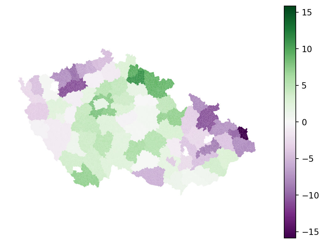
dtype: float64

The resulting Series can be merged with the elections_data, allowing us to map the spatial fixed effects.

1max_effect = fixed_effects.abs().max()
2elections_data.merge(
3    fixed_effects.to_frame("fixed_effect"),
4    left_on="okres",
5    right_index=True,
6    how="left",
7).plot(
8    "fixed_effect", legend=True, vmin=-max_effect, vmax=max_effect, cmap="PRGn"
).set_axis_off()

1: Identify the maximum fixed effect value based on absolute value to specify vmin and vmax values of the colormap.
2: Merge the fixed_effects to elections_data.
3: Merge requires a DataFrame, so convert it to one with a column named "fixed_effect".
4: Use the column "okres" from elections_data as a merge key.
5: Use the index of fixed_effects as a merge key.
6: Use the left join, keeping the structure of elections_data intact.
7: Plot the "fixed_effect".
8: Use max_effect to specify the extent of the colormap to ensure it had mid-point at 0.

Spatial regimes and spatial dependence

Where spatial fixed effects allow \(\alpha\) to change geographically (within each okres), spatial regimes allow \(\beta_k\) to change within the same regions. Spatial regimes cannot be done within statsmodels as they require more specialised treatment offered by the spreg package. Check the Spatial regimes sections of theSpatial Regression chapter from the Geographic Data Science with Python by Rey, Arribas-Bel, and Wolf (2023) for more details.

The same chapter also covers the modelling of spatial dependence using spreg. Both are considered advanced usage within this course but feel free to read through the materials yourself.

With spatial fixed effects, you were able to include spatial dimension in the model through a proxy variable, resulting in an improvement of adjusted \(R^2\) from 0.422 to 0.565 while also extracting the fixed effect of each okres. However, the model is still global. We are not able to determine how explanatory is education composition regionally.

Geographically weighted regression

Geographically Weighted Regression (GWR) overcomes the limitation of the OLS, which provides a single global estimate by examining how the relationship between a dependent variable and independent variable changes across different geographic locations. It does this by moving a search window through the dataset, defining regions around each regression point, and fitting a regression model to the data within each region. This process is repeated for all the sample points in the dataset, resulting in localized estimates. These local estimates can then be mapped to visualize variations in variable relationships at different locations. However, for a dataset with 6254 observations, like the one used here, GWR will fit 6254 weighted regression models. That can eventually pose a limitation when dealing with larger datasets, for which fitting the GWR can take too long.

Visually, you can imagine a spatial kernel being constructed around each location (point, specifically) where the kernel function defines its shape and bandwidth its size, as illustrated in Figure 1.

(a) Illustration of bandwidth and its relation to weight.

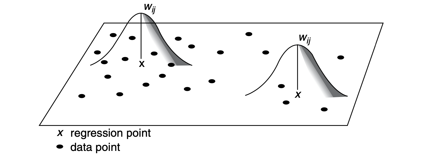
With kernels being the core of the GWR method, their specification significantly affects the resulting model. You can specify three parameters:

Kernel shape: The shape of the curve formed by the kernel. In mgwr package used here, "bisquare", "gaussian", and "exponential" kernels are supported.
Kernel size: The bandwidth distance specifying how large is the moving window.
Bandwidth adaptivity: Bandwidth can be either fixed, specified by the metric distance, where the moving window is essentially formed as a buffer around a point, or adaptive, specified by the number of nearest neighbours.

The details of the implications of the choices are beyond the scope of this lesson but are discussed in-depth by Fotheringham, Brunsdon, and Charlton (2002).

Fixed bandwidth

The method can be illustrated on a GWR using a fixed bandwidth and the default bi-square kernel.

Bandwidth selection

You may have some theoretically defined bandwidth (e.g. you know that you want to consider only locations closer than 25 km) or use cross-validation to find the optimal bandwidth programmatically. CV can be an expensive procedure as the selection procedure fits models based on different bandwidths and compares residuals to choose the one where those are minimised. mgwr has the mgwr.sel_bw.Sel_BW function that helps you with the search. But before using it (or any other mgwr function), you need to prepare the data in the correct form.

As mentioned above, the GWR assumes point locations as those are well-defined within the distance search (unlike polygons), so you need to extract centroids from geometries and get their coordinates.

1coords = elections_data.centroid.get_coordinates().values
coords

1: Create centroids, extract their coordinates and the underlying numpy array instead of a DataFrame.

array([[ -516260.37397642, -1168955.58212109],
       [ -556716.70278656, -1074526.68212735],
       [ -487873.89473542, -1123228.65302933],
       ...,
       [ -477659.1722107 , -1130589.89702433],
       [ -489845.39771121, -1104806.0459104 ],
       [ -477527.47958162, -1137135.07763038]])

Since mgwr is designed to work with numpy objects rather than pandas, extract both dependent and independent variables as arrays.

1y = elections_data[f"PetrPavel"].values.reshape(-1, 1)
2X = elections_data[independent_names[1:]].values

1: Get a column, extract its numpy representation and reshape it to an expected shape. The array should be two-dimensional.
2: Get a subset of columns and their array. Notice the omission of the first independent variable ([1:]). Unlike statsmodels, mgwr is not able to automatically deal with the interaction effects of independent variables while having an intercept. You therefore drop the first category and use the intercept in its place.

With the data ready, you can identify the optimal bandwidth. This step may take some time (probably minutes).

1sel_bw = mgwr.sel_bw.Sel_BW(coords, y, X, fixed=True)
2bw = sel_bw.search()
bw

1: Pass in coordinates, an array with dependent variable, an array with independent variables, and specify that you want a fixed bandwidth (in meters).
2: Initiate the search routine.

/home/runner/work/sds/sds/.pixi/envs/default/lib/python3.12/site-packages/spglm/iwls.py:37: LinAlgWarning: Ill-conditioned matrix (rcond=2.86955e-21): result may not be accurate.
  xtx_inv_xt = linalg.solve(xtx, xT)
/home/runner/work/sds/sds/.pixi/envs/default/lib/python3.12/site-packages/spglm/iwls.py:37: LinAlgWarning: Ill-conditioned matrix (rcond=1.1337e-20): result may not be accurate.
  xtx_inv_xt = linalg.solve(xtx, xT)
/home/runner/work/sds/sds/.pixi/envs/default/lib/python3.12/site-packages/spglm/iwls.py:37: LinAlgWarning: Ill-conditioned matrix (rcond=2.1118e-20): result may not be accurate.
  xtx_inv_xt = linalg.solve(xtx, xT)

np.float64(34156.84)

The optimal fixed bandwidth seems to be a bit more than 34 kilometres. You can pass it to the GWR function and fit the regression.

fixed_bandwidth = mgwr.gwr.GWR(
1    coords, y, X, bw=bw, fixed=True, name_x=independent_names[1:]
)
2results = fixed_bandwidth.fit()

1: Pass the data and bandwidth, specify that the bandwidth is fixed and optionally pass the names of each independent variable to be used in the report.
2: Fit the regression and save its results.

As before, you can use a summary method.

results.summary()

===========================================================================
Model type                                                         Gaussian
Number of observations:                                                6254
Number of covariates:                                                    14

Global Regression Results
---------------------------------------------------------------------------
Residual sum of squares:                                         472435.355
Log-likelihood:                                                  -22397.315
AIC:                                                              44822.630
AICc:                                                             44824.707
BIC:                                                             417891.662
R2:                                                                   0.423
Adj. R2:                                                              0.422

Variable                              Est.         SE  t(Est/SE)    p-value
------------------------------- ---------- ---------- ---------- ----------
Intercept                           36.341      9.252      3.928      0.000
undetermined                        -0.174      0.104     -1.676      0.094
incomplete_primary_education        -0.450      0.171     -2.632      0.008
lower_secondary_and_secondary_      -0.073      0.093     -0.786      0.432
further_education                    0.604      0.147      4.114      0.000
post_maturita_studies                0.991      0.223      4.433      0.000
bachelors_degree                     0.801      0.131      6.124      0.000
doctoral_degree                      0.860      0.237      3.624      0.000
masters_degree                       0.761      0.099      7.699      0.000
higher_vocational_education          1.369      0.160      8.539      0.000
higher_vocational_education_in       2.404      0.584      4.117      0.000
primary_education                   -0.290      0.101     -2.878      0.004
complete_secondary_vocational_       0.506      0.097      5.197      0.000
complete_secondary_general_edu       0.450      0.100      4.485      0.000

Geographically Weighted Regression (GWR) Results
---------------------------------------------------------------------------
Spatial kernel:                                          Fixed bisquare
Bandwidth used:                                                   34156.840

Diagnostic information
---------------------------------------------------------------------------
Residual sum of squares:                                         247717.876
Effective number of parameters (trace(S)):                          828.625
Degree of freedom (n - trace(S)):                                  5425.375
Sigma estimate:                                                       6.757
Log-likelihood:                                                  -20378.491
AIC:                                                              42416.232
AICc:                                                             42670.357
BIC:                                                              48008.716
R2:                                                                   0.698
Adjusted R2:                                                          0.652
Adj. alpha (95%):                                                     0.001
Adj. critical t value (95%):                                          3.339

Summary Statistics For GWR Parameter Estimates
---------------------------------------------------------------------------
Variable                   Mean        STD        Min     Median        Max
-------------------- ---------- ---------- ---------- ---------- ----------
Intercept                14.982    111.759   -762.050     29.479    632.521
undetermined              0.095      1.216     -5.568     -0.039      8.133
incomplete_primary_e      0.001      1.524     -6.517      0.067      7.218
lower_secondary_and_      0.146      1.144     -6.736     -0.003      7.741
further_education         0.562      1.614     -8.430      0.370     12.699
post_maturita_studie      0.874      1.686     -8.130      0.775      9.730
bachelors_degree          1.067      1.344    -10.384      0.969     11.854
doctoral_degree           1.021      2.255    -14.044      0.972     20.927
masters_degree            1.007      1.106     -3.376      0.896      7.763
higher_vocational_ed      1.086      1.549     -5.002      0.945     12.652
higher_vocational_ed      2.294      4.620    -20.287      2.507     32.090
primary_education         0.117      1.191     -7.115     -0.051      8.545
complete_secondary_v      0.624      1.182     -4.785      0.461      7.842
complete_secondary_g      0.617      1.133     -4.285      0.451      8.643
===========================================================================

The function fits GWR but also OLS for comparison and prints its results under the Global Regression Results section. You can see that the performance matches the first model done with statsmodels above. The performance of the GWR based on the adjusted \(R^2\) is 0.651, another improvement over the fixed effects OLS model. It is probably as good as it can be given the data on education can explain only a part of the election behaviour.

Apart from the global \(R^2\), GWR can report \(R^2\) per geometry, giving us further insights into where education is the driver of the election result and where you need to look for other causes.

1elections_data["local_r2"] = results.localR2
2elections_data.plot("local_r2", legend=True, vmin=0, vmax=1).set_axis_off()

1: Extract the array of local \(R^2\) and assign it as a column.
2: Plot the values on a map. The theoretical minimum is 0 and the maximum is 1.

Higher local \(R^2\) means that the model is able to use the data at each municipality and its surrounding areas to provide a result that is closer to the actual observed gain of Petr Pavel.

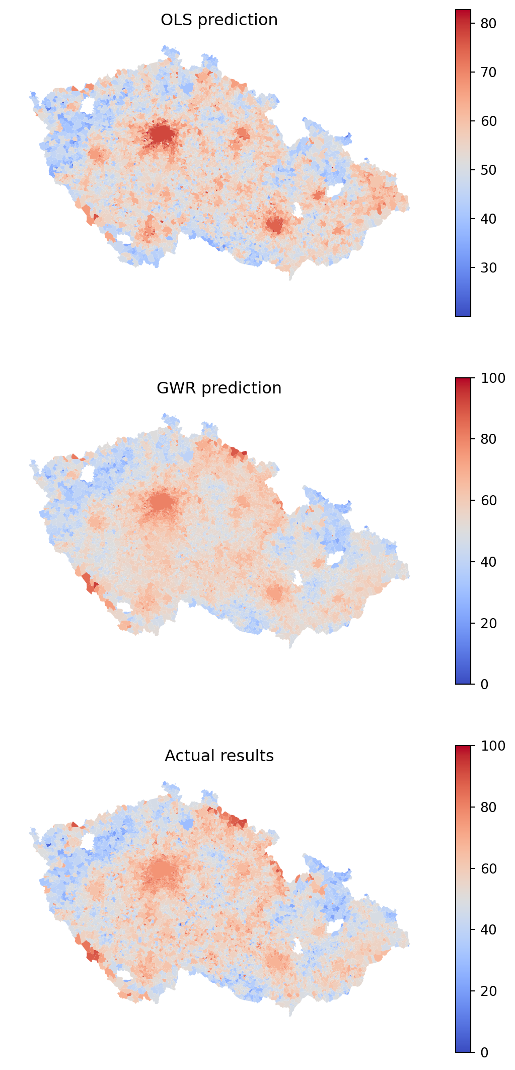
You can use the new GWR model and compare its predicted results with the OLS done first and the actual results.

Code

f, axs = plt.subplots(3, 1, figsize=(7, 14))
elections_data.plot(
    ols.predict(elections_data), legend=True, cmap="coolwarm", ax=axs[0]
)
elections_data.plot(
    results.predy.flatten(), legend=True, cmap="coolwarm", vmin=0, vmax=100, ax=axs[1]
).set_axis_off()

elections_data.plot(
    "PetrPavel", legend=True, cmap="coolwarm", vmin=0, vmax=100, ax=axs[2]
)
axs[0].set_title("OLS prediction")
axs[1].set_title("GWR prediction")
axs[2].set_title("Actual results")

axs[0].set_axis_off()
axs[1].set_axis_off()
axs[2].set_axis_off()

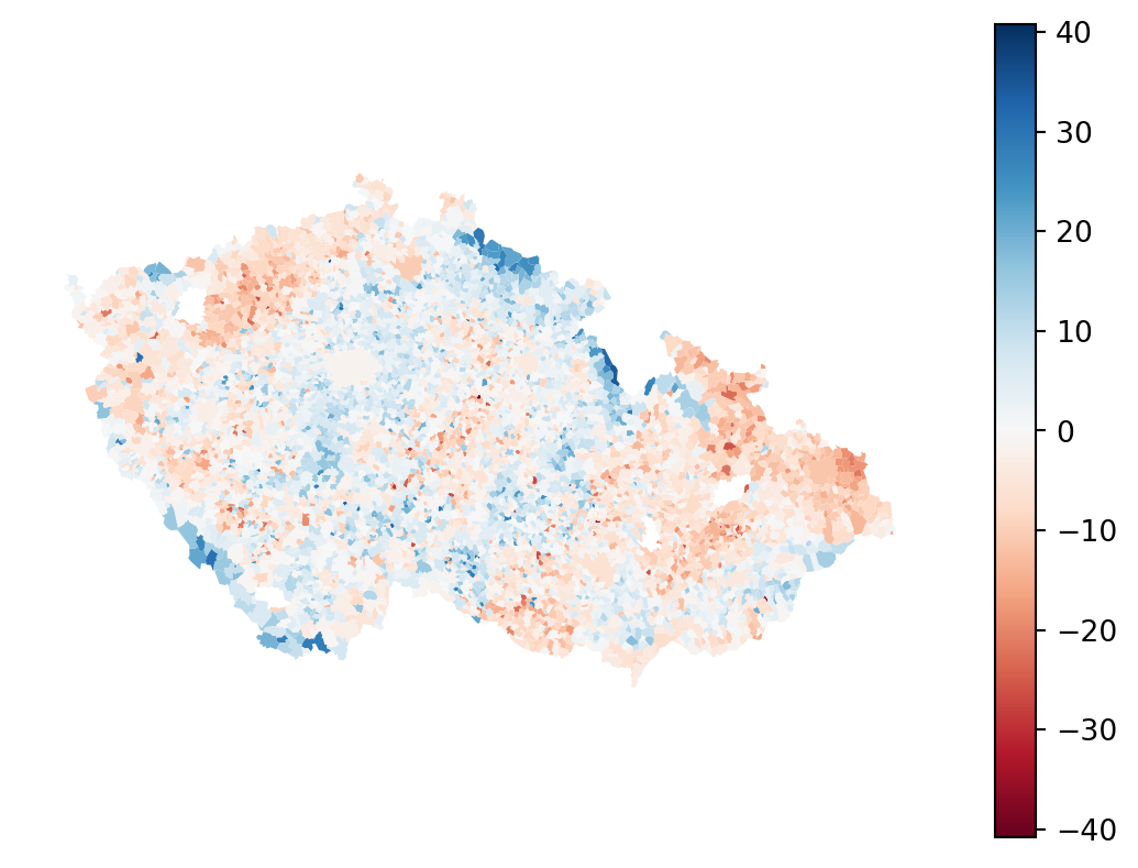
OLS prediction, GWR prediction, and the actual outcome

It is clear that the model is getting closer. Notice especially the mountains in the southwest and north of the country. You can check this even better by plotting residuals.

Code

f, axs = plt.subplots(2, 1, figsize=(7, 8))
elections_data.plot(
    "residual",
    legend=True,
    cmap="RdBu",
    vmin=-max_residual,
    vmax=max_residual,
    ax=axs[0],
)
elections_data.plot(
    results.resid_response.flatten(),
    legend=True,
    cmap="RdBu",
    vmin=-max_residual,
    vmax=max_residual,
    ax=axs[1],
)
axs[0].set_title("OLS residuals")
axs[1].set_title("GWR residuals")

axs[0].set_axis_off()
axs[1].set_axis_off()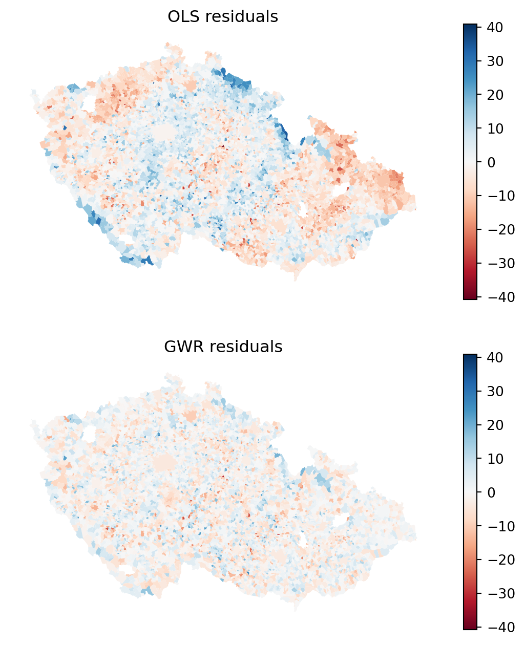

Apart from localised \(R^2\), GWR also contains localised \(\beta_k\) coefficients. While you can plot them directly (they are available as results.params), you should also understand whether the coefficients are statistically significant. For that, you first need to understand what is the critical value of \(t\). It is reported in the summary above but not available as an attribute.

The results object contains the adjusted alpha values for 0.1, 0.05 and 0.01 levels of significance:

results.adj_alpha

array([1.68954569e-03, 8.44772843e-04, 1.68954569e-05])

You can use the selected alpha value together with the results.critical_tval() method to get the critical value of \(t\).

1sig95 = results.adj_alpha[1]
2critical_t = results.critical_tval(alpha=sig95)
critical_t

1: Select 0.05 level of significance.
2: Derive \(t\).

np.float64(3.339312909177201)

If a coefficient estimate has an absolute value of \(t\) greater than 3.33, then it is statistically significant. You can use this level to mask out the coefficients on the maps below making a distinction between significant and non-significant values.

significant = np.abs(results.tvalues) > critical_t

fig, axs = plt.subplots(4, 3, figsize=(9, 9))
axs = axs.flatten()
for i, name in enumerate(independent_names[1:-1]):
    significant_mask = significant[:, i + 1]
    elections_data.plot(results.params[:, i + 1], cmap="plasma", ax=axs[i])
    elections_data[~significant_mask].plot(color="white", ax=axs[i], alpha=.9)
    axs[i].set_title(name[:20], fontdict={'fontsize': 8})
    axs[i].set_axis_off()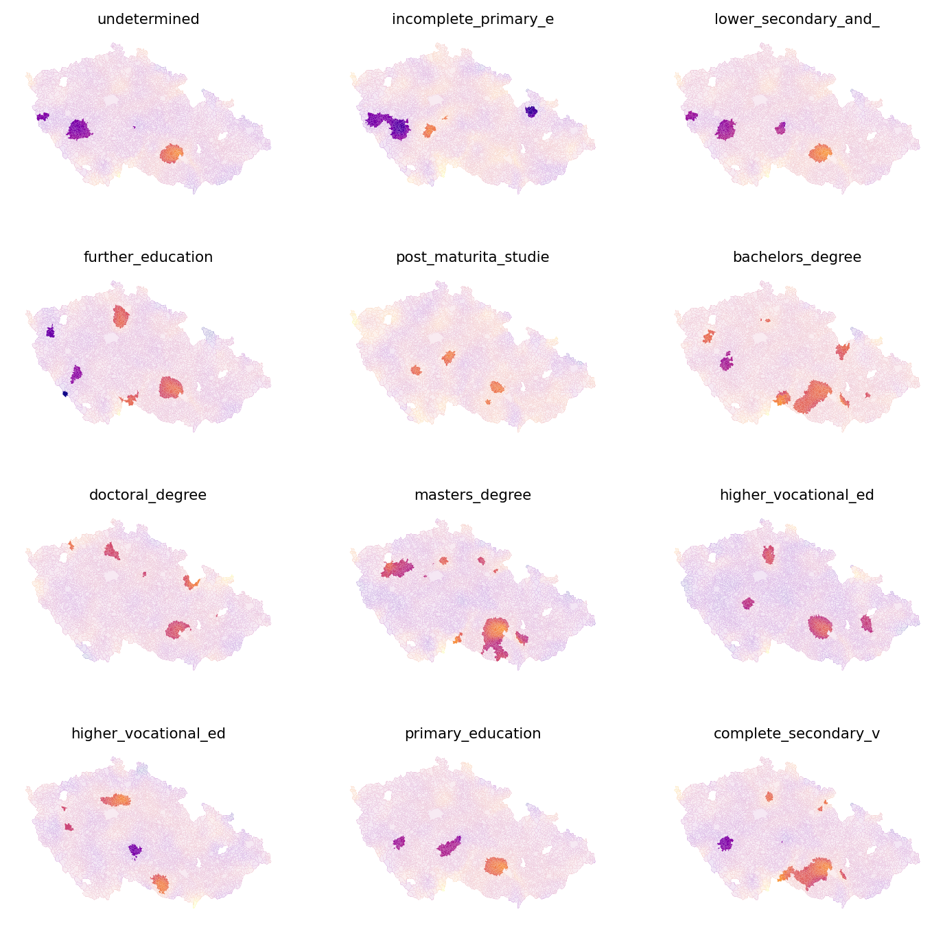

It seems that the coefficients are significant only in some areas, so you need to be careful when drawing conclusions here. This can be due to a lack of relationship or a small sample size. Try for yourself how the significance changes if you increase the bandwidth. But be careful as too large a bandwidth may miss regional differences and a bandwidth that would cover the whole country would be equal to the OLS model.

Adaptive bandwidth

If you’d like to use the adaptive bandwidth, you can use same tools. Just specify fixed=False in both Sel_BW and GWR.

sel_bw = mgwr.sel_bw.Sel_BW(coords, y, X, fixed=False)
bw = sel_bw.search()

adaptive = mgwr.gwr.GWR(coords, y, X, bw=bw, fixed=False, name_x=independent_names[1:])
results_adaptive = adaptive.fit()

Additional reading

Have a look at the chapter Spatial Regression from the Geographic Data Science with Python by Rey, Arribas-Bel, and Wolf (2023) for more details and some other extensions.

If you’d like to learn the details of GWR, Geographically Weighted Regression by Fotheringham, Brunsdon, and Charlton (2002) is a good start.

Acknowledgements

The first part of this section loosely follows the Spatial Regression chapter from the Geographic Data Science with Python by Rey, Arribas-Bel, and Wolf (2023). The section of GWR is inspired by the Spatial Modelling for Data Scientists course by Rowe and Arribas-Bel (2023).

References

Fotheringham, A Stewart, Chris Brunsdon, and Martin Charlton. 2002. Geographically Weighted Regression: The Analysis of Spatially Varying Relationships. John Wiley & Sons.

Rey, Sergio, Dani Arribas-Bel, and Levi John Wolf. 2023. Geographic Data Science with Python. Chapman & Hall/CRC Texts in Statistical Science. London, England: Taylor & Francis.

Rowe, Francisco, and Daniel Arribas-Bel. 2023. “Spatial Modelling for Data Scientists.” https://smds-book.github.io/smds/.