Spatial evaluation and model architecture

Linear regression, covered in the previous chapter, is often seen as an entry method to enter the world of supervised machine learning. However, not every phenomenon can be explained using a linear relationship, and not everything is a regression. For the former, you need to use methods that have a bit more complicated math behind them (but often the same Python API). For the latter, you will often need to look for classification models. Both of these options are covered in this course, with non-linear regression models in this session and classification in the next one. Today, you’ll focus on learning the API and the key principles of supervised machine learning with scikit-learn and especially on spatial evaluation of model performance. To a degree, it is a continuation of the work covered last time, but there are some new things here and there.

This is not an introduction to ML

Note that this material does not aim to cover an introduction to machine learning thoroughly. There are other, much better materials for that. One of them can be scikit-learn’s User guide, but I am sure you will find one that suits you.

import esda
import geopandas as gpd
import matplotlib.pyplot as plt
import numpy as np
import pandas as pd
import pyinterpolate
from libpysal import graph
from sklearn import ensemble, metrics, model_selection, svm

Data

Let’s stick to a similar type of data you were working with in the previous chapter on linear regression. The data you will be working with today is, once again, representing municipalities in Czechia but this time your task will not be prediction of election results but the rate of executions (of any kind, not only those related to mortgages). The dataset is representing the proportion of population aged 15 and above in each municipality with at least one court mandated execution during the Q3 of 2024, coming from mapazadluzeni.cz by PAQ Research. The CSV is only slightly pre-processed to contain only relevant information.

executions = pd.read_csv(
    "https://martinfleischmann.net/sds/tree_regression/data/czechia_executions_q3_2024.csv"
)
executions.head()

	kod_obce	nazev_obce	kod_orp	nazev_orp	kod_okresu	nazev_okresu	kod_kraje	nazev_kraje	podil_osob_v_exekuci
0	500011	Želechovice nad Dřevnicí	7213	Zlín	40851	Zlín	3131	Zlínský kraj	3.1
1	500020	Petrov nad Desnou	7111	Šumperk	40819	Šumperk	3123	Olomoucký kraj	4.6
2	500046	Libhošť	8115	Nový Jičín	40894	Nový Jičín	3140	Moravskoslezský kraj	2.1
3	500062	Krhová	7210	Valašské Meziříčí	40843	Vsetín	3131	Zlínský kraj	1.9
4	500071	Poličná	7210	Valašské Meziříčí	40843	Vsetín	3131	Zlínský kraj	1.3

Alternative

Instead of reading the file directly off the web, it is possible to download it manually, store it on your computer, and read it locally. To do that, you can follow these steps:

Download the file by right-clicking on this link and saving the file
Place the file in the same folder as the notebook where you intend to read it
Replace the code in the cell above with:

executions = pd.read_csv(
    "czechia_executions_q3_2024.csv",
)

You have your target variable. The models will try to predict it based on a set of independent variables of which the first is the proportion of votes for Andrej Babiš, a candidate often marked as a populist or belonging to the anti-system movement (although not as strongly as some other parties in the country). You can read this data from the chapter on autocorrelation. The dataset also provides geometries of individual municipalities.

elections = gpd.read_file(
    "https://martinfleischmann.net/sds/autocorrelation/data/cz_elections_2023.gpkg"
)
elections = elections.set_index("name")
elections.head()

	nationalCode	PetrPavel	AndrejBabis	sourceOfName	geometry
name
Želechovice nad Dřevnicí	500011	61.73	38.26	Český úřad zeměměřický a katastrální	MULTIPOLYGON (((-518835.63 -1170505.52, -51790...
Petrov nad Desnou	500020	49.07	50.92	Český úřad zeměměřický a katastrální	MULTIPOLYGON (((-559207.18 -1075123.25, -55624...
Libhošť	500046	47.78	52.21	Český úřad zeměměřický a katastrální	MULTIPOLYGON (((-486502.29 -1123694.06, -48717...
Krhová	500062	58.79	41.20	Český úřad zeměměřický a katastrální	MULTIPOLYGON (((-494514.83 -1136457.23, -49539...
Poličná	500071	58.20	41.79	Český úřad zeměměřický a katastrální	MULTIPOLYGON (((-499678.51 -1143457.52, -49799...

Second set of independent variables are reflecting education profile. It is the same dataset you have used last week. This time, you will use only a subset though.

education = pd.read_csv(
    "https://martinfleischmann.net/sds/regression/data/education.csv"
)
education.head()

	uzemi_kod	without_education	undetermined	incomplete_primary_education	lower_secondary_and_secondary_education	further_education	post_maturita_studies	bachelors_degree	doctoral_degree	masters_degree	higher_vocational_education	higher_vocational_education_in_a_conservatory	primary_education	complete_secondary_vocational_education	complete_secondary_general_education	okres
0	500011	0.570704	3.741281	1.141408	34.242232	1.775523	0.507292	2.853519	0.634115	12.935954	1.395054	0.126823	11.350666	17.945466	10.779962	Zlín
1	500020	0.885827	3.346457	1.968504	40.157480	2.066929	0.885827	1.771654	0.492126	6.299213	1.574803	0.000000	15.059055	16.338583	9.153543	Šumperk
2	500046	0.359195	3.232759	0.790230	39.152299	2.514368	0.790230	3.520115	0.215517	10.632184	1.364943	0.143678	9.770115	15.301724	12.212644	Nový Jičín
3	500062	0.238237	3.573556	1.072067	32.757594	2.084574	1.131626	3.037522	0.178678	13.281715	0.714711	0.119119	11.316260	18.701608	11.792734	Vsetín
4	500071	0.412939	2.890571	1.238816	34.067447	1.720578	0.757054	3.028217	0.137646	11.080523	0.894701	0.000000	9.772884	20.027529	13.971094	Vsetín

On top of that, you will use the average population age and a proportion of divorced in the population.

age_divorces = pd.read_csv(
    "https://martinfleischmann.net/sds/tree_regression/data/cz_age_divorces_2021.csv"
)
age_divorces.head()

	uzemi_kod	divorced	mean_age
0	500011	0.047056	45.528343
1	500020	0.057741	44.782427
2	500046	0.037081	42.127722
3	500062	0.046040	42.579208
4	500071	0.040210	43.869464

Given each dataset is in its own (Geo)DataFrame now, the first thing is to merge them together to have a single GeoDataFrame to work with throughout the notebook. Each of them has a column representing code of each municipality, allowing use to easily merge the data together.

executions_data = (
    elections
    .merge(executions, left_on="nationalCode", right_on="kod_obce")
    .merge(education, left_on="nationalCode", right_on="uzemi_kod")
    .merge(age_divorces, left_on="nationalCode", right_on="uzemi_kod")
    )
executions_data.head()

	nationalCode	PetrPavel	AndrejBabis	sourceOfName	geometry	kod_obce	nazev_obce	kod_orp	nazev_orp	kod_okresu	...	masters_degree	higher_vocational_education	higher_vocational_education_in_a_conservatory	primary_education	complete_secondary_vocational_education	complete_secondary_general_education	okres	uzemi_kod_y	divorced	mean_age
0	500011	61.73	38.26	Český úřad zeměměřický a katastrální	MULTIPOLYGON (((-518835.63 -1170505.52, -51790...	500011	Želechovice nad Dřevnicí	7213	Zlín	40851	...	12.935954	1.395054	0.126823	11.350666	17.945466	10.779962	Zlín	500011	0.047056	45.528343
1	500020	49.07	50.92	Český úřad zeměměřický a katastrální	MULTIPOLYGON (((-559207.18 -1075123.25, -55624...	500020	Petrov nad Desnou	7111	Šumperk	40819	...	6.299213	1.574803	0.000000	15.059055	16.338583	9.153543	Šumperk	500020	0.057741	44.782427
2	500046	47.78	52.21	Český úřad zeměměřický a katastrální	MULTIPOLYGON (((-486502.29 -1123694.06, -48717...	500046	Libhošť	8115	Nový Jičín	40894	...	10.632184	1.364943	0.143678	9.770115	15.301724	12.212644	Nový Jičín	500046	0.037081	42.127722
3	500062	58.79	41.20	Český úřad zeměměřický a katastrální	MULTIPOLYGON (((-494514.83 -1136457.23, -49539...	500062	Krhová	7210	Valašské Meziříčí	40843	...	13.281715	0.714711	0.119119	11.316260	18.701608	11.792734	Vsetín	500062	0.046040	42.579208
4	500071	58.20	41.79	Český úřad zeměměřický a katastrální	MULTIPOLYGON (((-499678.51 -1143457.52, -49799...	500071	Poličná	7210	Valašské Meziříčí	40843	...	11.080523	0.894701	0.000000	9.772884	20.027529	13.971094	Vsetín	500071	0.040210	43.869464

5 rows × 33 columns

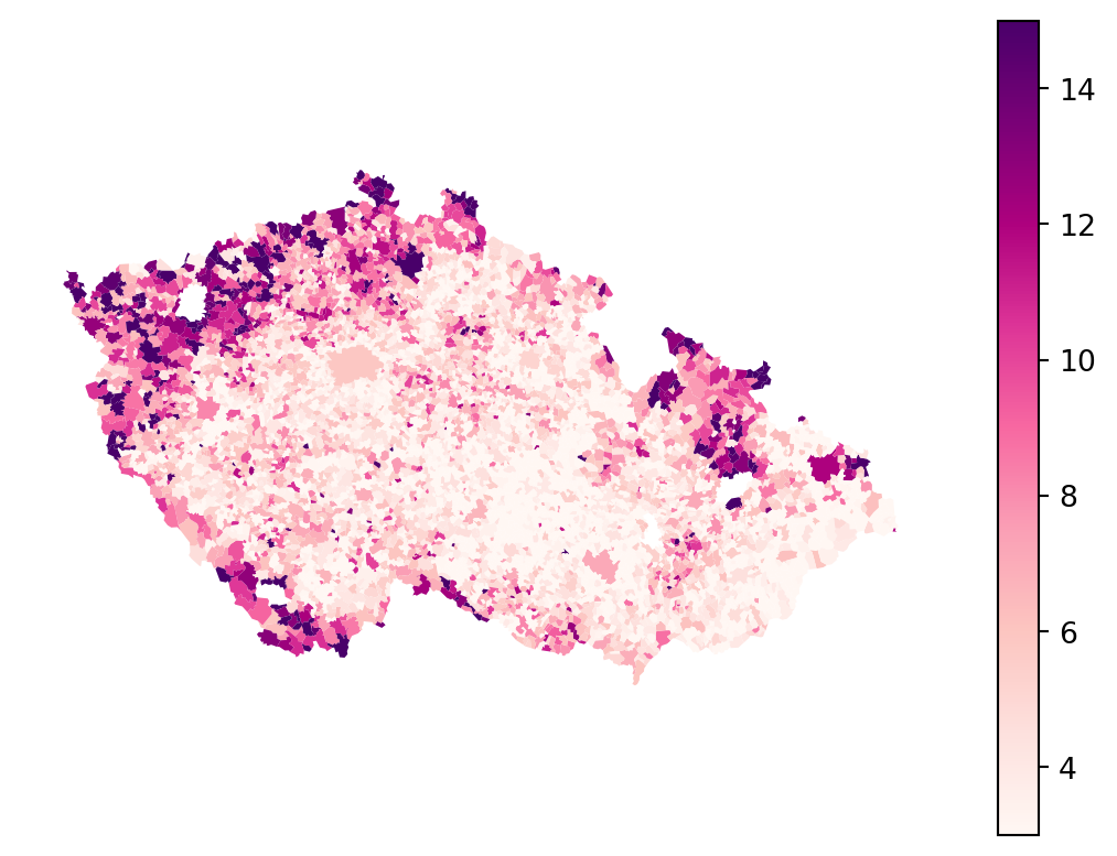
You can notice that some of the columns are in Czech. The important one is "podil_osob_v_exekuci", which stands for a ratio of people with a execution. Check how does the spatial distribution looks like, to get a sense.

executions_data.plot(
    "podil_osob_v_exekuci",
    legend=True,
1    vmin=3,
    vmax=15,
    cmap="RdPu",
).set_axis_off()

1: Specifying minimum and maximum for the colormap based on the values used by PAQ Research. It helps filtering out outliers.

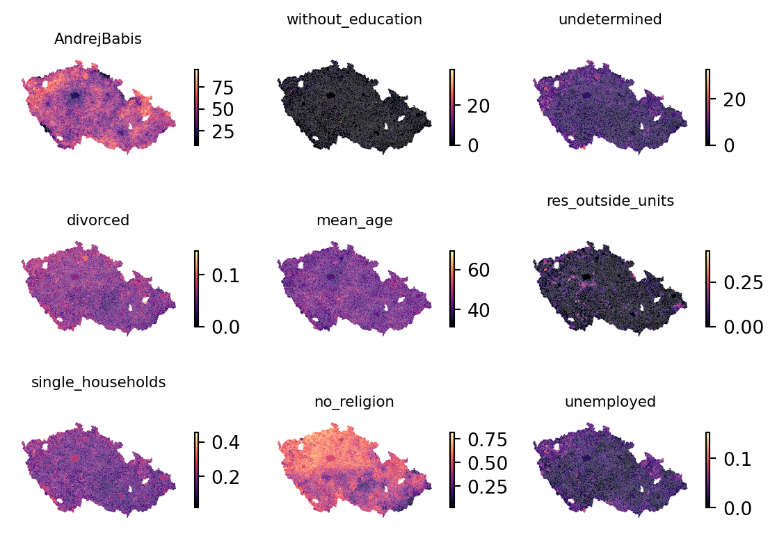
Proportion of population with executions

The executions_data GeoDataFrame has obviously more columns than we need. For the modelling purpose, select a subset of variables to treat as independent, explanatory. The election results of Andrej Babiš, three columns representing education levels, mean age and divorced rate.

independent_variables = [
    "AndrejBabis",
    "undetermined",
    "masters_degree",
    "primary_education",
    "mean_age",
    "divorced",
]

You can briefly check how each looks on a map and compare them to the distribution of executions.

fig, axs = plt.subplots(3, 2)
for variable, ax in zip(independent_variables, axs.flatten()):
    executions_data.plot(
        variable,
        ax=ax,
        cmap="magma",
        legend=True,
1        legend_kwds=dict(shrink=0.5),
    )
    ax.set_title(variable, fontdict={"fontsize": 8})
    ax.set_axis_off()

1: Make the colorbar half the size for a better looking plot.

Spatial distribution of independent variables

Machine learning 101

As mentioned above, this material is not meant to provide exhaustive introduction to machine learning. Yet, some basics shall be explained. Start with storing independent variables and a target variable separately.

independent = executions_data[independent_variables]
target = executions_data["podil_osob_v_exekuci"]

Train-test split

Some data are used to train the model, but the same data cannot be used for evaluation. The models tend to learn those exact values, and the performance metrics derived from training data show a much higher score than the model can on unseen data. One way around this is to split the dataset into two parts - train and test. The train part is used to train the model. However, the test part is left out of training and is later used to evaluate performance without worrying that any of the data points were seen by the model before.

scikit-learn offers handy function to split the data into train and test parts, dealing with both dependent and independent variables at the same time.

1X_train, X_test, y_train, y_test = model_selection.train_test_split(
    independent, target, test_size=0.2, random_state=0
)
X_train.head()

1: X and y are not very explanatory variable names but they are used in ML so often to reflect independent (X) and dependent (y) variables that everyone knows what they mean. You’ll see the same naming across scikit-learn’s documentation.

	AndrejBabis	undetermined	masters_degree	primary_education	mean_age	divorced
4126	34.31	4.103842	12.849089	10.607054	46.251550	0.061366
6100	26.66	11.016949	10.593220	6.991525	40.045872	0.073394
5222	60.52	3.061224	4.081633	13.265306	43.833333	0.045833
1788	44.15	4.856512	9.602649	13.355408	43.606174	0.050514
546	39.88	5.284435	10.511118	11.059775	43.974484	0.056744

You can check that X_*, containing independent variables is split into two parts, one with 80% of the data and the other with remaining 20%. Completely randomly.

X_train.shape, X_test.shape

((5003, 6), (1251, 6))

Training

While there is a large number of ML models available, your goal at the moment is not to understand which ML model is better and how to fine-tune it but how to evaluate it using the spatial dimension. So, let’s not complicate the situation and stick to one of the common models - random forest.

Random forest regressor is implemented within the ensemble module of the scikit-learn and has the API you should already be familiar with. Get the training data and fit the baseline model.

basic_model = ensemble.RandomForestRegressor(n_jobs=-1, random_state=0)
basic_model.fit(X_train, y_train)

RandomForestRegressor(n_jobs=-1, random_state=0)

In a Jupyter environment, please rerun this cell to show the HTML representation or trust the notebook.
On GitHub, the HTML representation is unable to render, please try loading this page with nbviewer.org.

n_jobs=-1 specifies that the algorithm should use all available cores. Otherwise, it runs in a single thread only. There are also some model parameters to play with but more on that below.
The first argument is a 2-D array of independent variables, and the second is a 1-D array of labels you want to predict.

Predicting

The trained model can be directly used to predict the value, the proportion of executions. Normally, you do the prediction using the unseen portion of the data from the train-test split.

pred_test = basic_model.predict(X_test)
pred_test

array([4.868, 6.952, 4.479, ..., 3.188, 2.937, 6.721])

The output is a simple numpy array aligned with the values from X_test. What this array is mostly used for is the model evaluation.

Evaluation

Evaluation is usually composed a series of measurements comparing the expected and predicted values and assessing how close the result is. Regression problems typically use \(R^2\), mean absolute error, or root mean squared error among others. Let’s stick to these three for now. All are directly implemented in scikit-learn.

R-squared

\(R^2\) is a measure you should already be familiar with from the previous session on linear regression. It expresses the proportion of variation of the target variable that could be predicted from the independent variables.

r2 = metrics.r2_score(y_test, pred_test)
r2

0.5590843309809401

This baseline model is able to explain about 56% of variation. Not bad, given the limited data and no fine-tuning.

Mean absolute error

The name kind of says it all. The mean absolute error (MAE) reports how far, on average, is the predicted value from the expected one. All that directly in the units of the original target variable, making it easy to interpret.

mean_absolute_error = metrics.mean_absolute_error(y_test, pred_test)
mean_absolute_error

1.661047961630696

Here, you can observe that the error is about 1.6% on average. But given the average rate of executions is 4.95%, it is quite a bit of spread.

Root mean squared error

Root mean squared error (RMSE) is a very similar metric but it is more sensitive to larger errors. Therefore, if there is a smaller proportion of observations that are very off, RMSE will penalise the resulting performance metric more than MAE.

rmse = metrics.root_mean_squared_error(y_test, pred_test)
rmse

2.555496623673198

It is a bit larger than MAE in this case, meaning that there are outliers with exceptionally high residuals. You’ll be looking at multiple models and evaluations, so let’s start building a summary allowing simple reporting and comparison.

summary = f"""\
Evaluation metrics
==================
Random Forest:
  R2:   {round(r2, 3)}
  MAE:  {round(mean_absolute_error, 3)}
  RMSE: {round(rmse, 3)}
1"""
print(summary)

1: The summary is using a multiline f-strings to fill the values within the string.

Evaluation metrics
==================
Random Forest:
  R2:   0.559
  MAE:  1.661
  RMSE: 2.555

Cross validation

Now, if you want to plot the predicted labels on a map, you can do that reliably only for the test sample. The training sample was seen by the model and would not be representative of model capabilities.

executions_data.assign(
    pred_test=pd.Series(pred_test, index=X_test.index)
).plot("pred_test", legend=True).set_axis_off()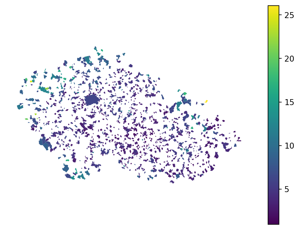

Working with this would be a bit tricky if we want to look into the spatial dimension of the model error.

However, you can create a map using the complete sample, just not using exactly the same model for all its parts. Welcome cross-validated prediction.

Cross-validated (CV) prediction splits the dataset (before you divided it into train and test) into a small number of parts and trains a separate model to predict values for each of them. In the example below, it creates five equally-sized parts and then takes four of them as train part to train a model that is used to predict values on the fifth one. Then, it switches the one that is left out and repeats the process until there are predicted values for every part. The resulting prediction should not contain any data leakage between train and test samples. However, as described below, that is not always the case when dealing with spatial data.

pred_cross_val = model_selection.cross_val_predict(
    basic_model,
    independent,
    target,
    n_jobs=-1,
)
pred_cross_val

array([3.523, 4.533, 2.436, ..., 2.866, 2.166, 2.796])

The array pred_cross_val now has the same length as the original data and can be therefore plotted on a full map.

executions_data.plot(pred_cross_val, legend=True).set_axis_off()

Cross-validated prediction on the full dataset

Cross-validation also allows you to assess the quality of the model more reliably, minimising the effect of sampling on the metric. You can simply measure the performance on the full array taking into account every of the five folds.

r2_cross_val = metrics.r2_score(
    target, pred_cross_val
)
mae_cross_val = metrics.mean_absolute_error(
    target, pred_cross_val
)
rmse_cross_val = metrics.root_mean_squared_error(
    target, pred_cross_val
)

summary += f"""\
Random Forest (k-fold metrics):
  R2:   {round(r2_cross_val, 3)}
  MAE:  {round(mae_cross_val, 3)}
  RMSE: {round(rmse_cross_val, 3)}
"""
print(summary)

Evaluation metrics
==================
Random Forest:
  R2:   0.559
  MAE:  1.661
  RMSE: 2.555
Random Forest (k-fold metrics):
  R2:   0.527
  MAE:  1.695
  RMSE: 2.62

These results are not wildly off but the performance dropped a bit. The smaller the dataset (and this one is pretty small) the higher the effect of train-test split could be. Let’s refer to the cross-validated metrics as more reliable representation of the performance of the baseline model here.

Residuals

Another positive aspect of cross validation is that is allows use to retrieve a full sample of residuals. Unlike in linear regression, where residuals are part of the model, here you have to compute them yourself as a difference between expected and a predicted value.

residuals = (target - pred_cross_val)
residuals.head()

0   -0.423
1    0.067
2   -0.336
3   -0.738
4   -1.174
Name: podil_osob_v_exekuci, dtype: float64

Negative values mean the model have over-predicted the value, while the positive one means under-prediction. The optimal is zero. Check the residuals on a map.

1minmax = residuals.abs().std()
executions_data.plot(
    residuals,
2    vmin=-minmax * 5,
    vmax=minmax * 5,
    cmap="RdBu",
    legend=True,
).set_axis_off()

1: Getting the standard deviation of the absolute value of residuals to help to reasonably stretch the colormap.
2: Get the minimum and maximum of the colormap as 5 standard deviations below or above zero.

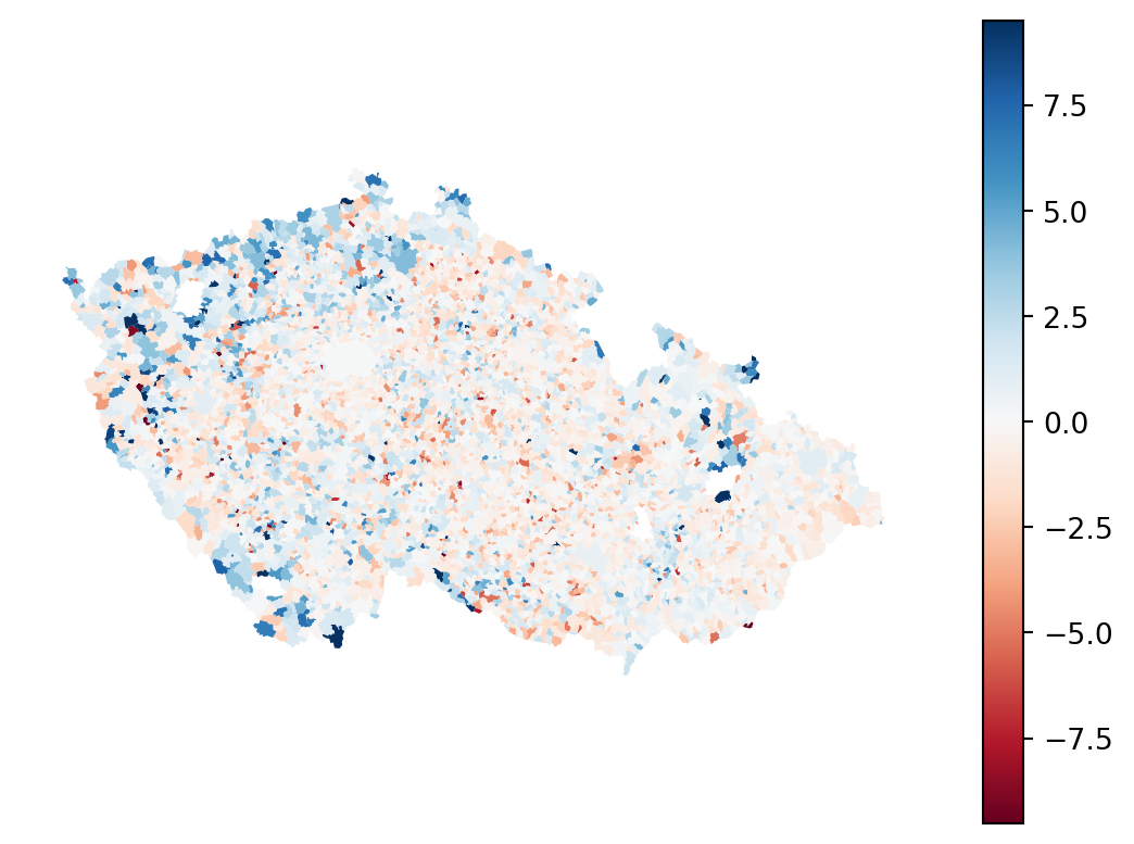
The spatial pattern of error signifies issues, you should know that from the last session. You can optionally use some strategies covered there to mitigate it. Today, let’s look and more advanced spatial evaluation of the model performance.

Spatial evaluation

The metrics reported above are global. A single value per model but the map indicates that this varies in space. Let’s see how.

Spatially stratified metrics

Global metrics can be computed on regional subsets. We have an information about okres (county) and can try computing the metrics for each individual okres. To make it all a bit easier, assign the cross-validated prediction as a new column.

executions_data["prediction"] = pred_cross_val

Using groupby, you can group the data by "okres" and check the metric within each one. Better to measure metrics derived from real values than \(R^2\) as the latter is not well comparable across different datasets (each okres would be its own dataset in this logic).

1grouped = executions_data.groupby("okres")[
    ["podil_osob_v_exekuci", "prediction"]
]

2block_mae = grouped.apply(
    lambda group: metrics.mean_absolute_error(
        group["podil_osob_v_exekuci"], group["prediction"]
    )
)
block_rmse = grouped.apply(
    lambda group: metrics.root_mean_squared_error(
        group["podil_osob_v_exekuci"], group["prediction"]
    )
)

1: Group by "okres" and selected a subset of relevant columns to work on.
2: Use apply together with the lambda function defined on the fly to pass the relevant columns of each group as parameters of the metric function.

As a result, you now have two Series with the metric per okres.

block_mae.head()

okres
Benešov        1.469640
Beroun         1.106306
Blansko        1.159198
Brno-město     2.919000
Brno-venkov    1.237567
dtype: float64

Let’s concatenate them together to a single DataFrame with proper column names.

spatial_metrics = pd.concat([block_mae, block_rmse], axis=1)
spatial_metrics.columns = ["block_mae", "block_rmse"]
spatial_metrics.head(3)

	block_mae	block_rmse
okres
Benešov	1.469640	2.320084
Beroun	1.106306	1.386071
Blansko	1.159198	1.639552

And merge with the original data. The spatial metrics cannot be simply assigned as new columns as they are much shorter - only one value per okres. You need to merge on the okres values to assign it as new columns.

executions_data = executions_data.merge(
    spatial_metrics, left_on="okres", right_index=True
)
executions_data.head(3)

	nationalCode	PetrPavel	AndrejBabis	sourceOfName	geometry	kod_obce	nazev_obce	kod_orp	nazev_orp	kod_okresu	...	primary_education	complete_secondary_vocational_education	complete_secondary_general_education	okres	uzemi_kod_y	divorced	mean_age	prediction	block_mae	block_rmse
0	500011	61.73	38.26	Český úřad zeměměřický a katastrální	MULTIPOLYGON (((-518835.63 -1170505.52, -51790...	500011	Želechovice nad Dřevnicí	7213	Zlín	40851	...	11.350666	17.945466	10.779962	Zlín	500011	0.047056	45.528343	3.523	1.264901	1.664545
1	500020	49.07	50.92	Český úřad zeměměřický a katastrální	MULTIPOLYGON (((-559207.18 -1075123.25, -55624...	500020	Petrov nad Desnou	7111	Šumperk	40819	...	15.059055	16.338583	9.153543	Šumperk	500020	0.057741	44.782427	4.533	1.733577	2.874693
2	500046	47.78	52.21	Český úřad zeměměřický a katastrální	MULTIPOLYGON (((-486502.29 -1123694.06, -48717...	500046	Libhošť	8115	Nový Jičín	40894	...	9.770115	15.301724	12.212644	Nový Jičín	500046	0.037081	42.127722	2.436	0.722556	0.926253

3 rows × 36 columns

Let’s see how the performance differs across space.

fig, axs = plt.subplots(2, 1)
for i, metric in enumerate(["block_mae", "block_rmse"]):
    executions_data.plot(metric, ax=axs[i], legend=True, cmap="cividis")
    axs[i].set_title(metric, fontdict={"fontsize": 8})
    axs[i].set_axis_off()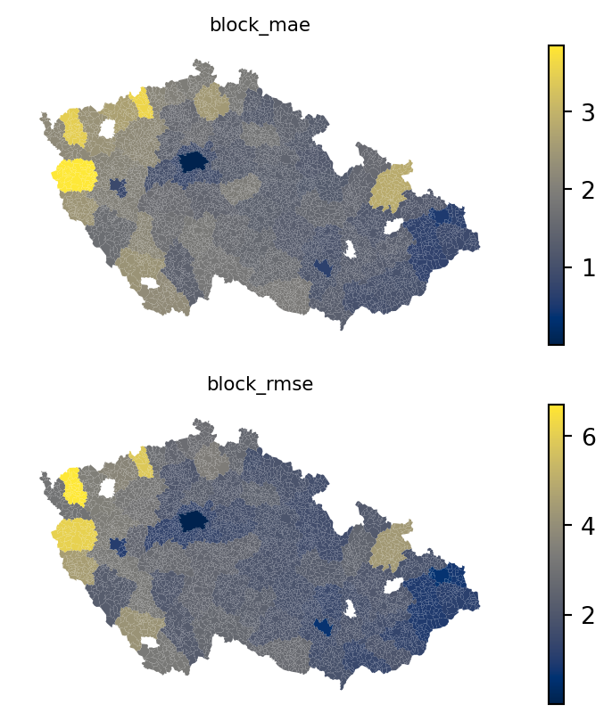

MAE and RSME measured per each aggregated region

The spatial variation is evident. What is also evident are the boundaries between individual okres’s, suggesting a MAUP issue. At the same time, such an aggregation may not always be available.

The better option is to measure the spatial metrics using the Graph. You can define neighborhoods and measure the metric in each neighborhood individually, reporting a unique value per each focal geometry. In this case, you can assume that the daily mobility is not limited to neighbouring municipalities only, so let’s get a K-nearest neighbors with 100 neighbor (median number of municipalities in the okres is 79, so it should cover roughly similar scale). Using very small neighborhoods may result in the metrics jumping up and down erratically due to sampling issue.

knn100 = graph.Graph.build_knn(
1    executions_data.set_geometry(executions_data.centroid), 100
2).assign_self_weight()

3executions_data["spatial_mae"] = knn100.apply(
    executions_data[["podil_osob_v_exekuci", "prediction"]],
    lambda df: metrics.mean_absolute_error(
        df["podil_osob_v_exekuci"], df["prediction"]
    ),
)
executions_data["spatial_rmse"] = knn100.apply(
    executions_data[["podil_osob_v_exekuci", "prediction"]],
    lambda df: metrics.root_mean_squared_error(
        df["podil_osob_v_exekuci"], df["prediction"]
    ),
)

1: Set geometry to centroids (on-the-fly) as the KNN constructor requires point geometries.
2: Assign self-weight to 1, effectively including focal geometry in its own neighbourhood.
3: Graph.apply works as an overlapping groupby.apply. You just need to give it the actual data as the first argument. Remember that the graph contains only the information about the relationship.

You can map the results again, observing much smoother transitions between low and high values, minimising boundary aspect of MAUP (the scale aspect is still present).

fig, axs = plt.subplots(2, 1)
for i, metric in enumerate(["spatial_mae", "spatial_rmse"]):
    executions_data.plot(metric, ax=axs[i], legend=True, cmap="cividis")
    axs[i].set_title(metric, fontdict={"fontsize": 8})
    axs[i].set_axis_off()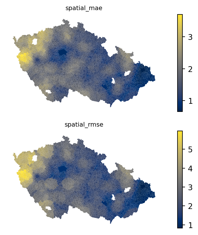

MAE and RSME measured within 100 nearest neighbors. Notice the more visible artifacts of large errors in the RSME map caused by the penalisation.

With these data, you can do any of the spatial analysis you are used to, like extracting local clusters of low or high performance or fixing the model to avoid these artifacts.

Spatial dependency of error

Let’s now focus on a direct spatial assessment of residuals. The map of residuals above indicates that there is some spatial structure to unpack, so let’s dive into the assessment of the spatial dependency of the model error.

Variogram

Let’s check the spread of the assumed autocorrelation. Is the dependency relevant only locally, regionally or nationally? To answer this question, you can build an experimental variogram, like you did when dealing with kriging. The variogram should then indicate the extent of autocorrelation.

Remember, that pyinterpolate assumes data in a specific structure, so let’s quickly prepare it. For details check the interpolation chapter.

input_data = np.hstack(
    [
        executions_data.centroid.get_coordinates(),
1        residuals.abs().values.reshape(-1, 1),
    ]
)

1: Use absolute value of residuals to assess the autocorrelation of model imprecision, irrespective of the direction.

Build the variogram, ideally covering the width of the whole country.

exp_semivar = pyinterpolate.build_experimental_variogram(
    input_array=input_data,
1    step_size=10_000,
2    max_range=490_000,
)

1: Step size set to 10km.
2: Max range is 490km, which is the rough width of the dataset.

With the built semivariogram, you can explore its plot.

exp_semivar.plot(plot_covariance=False)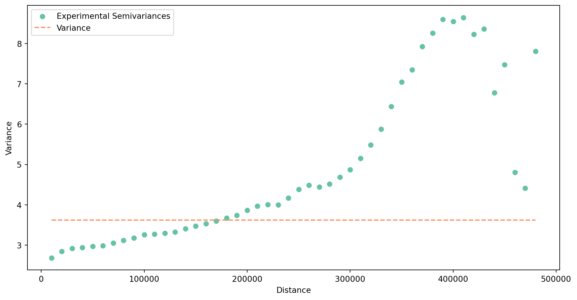

The semivariance tends to grow nearly across the whole range, indicating that the autocorrelation does not disappear when considering larger regions. More, it seems that there is difference in performance across large parts of the country. In any case, the results clearly suggests that the model has a troubles with spatial heterogeneity of the relationship between independent variables and the target one.

LISA on residuals

One approach of determining spatial dependence of the residuals you are already familiar with is measuring local indicators of spatial autocorrelation. The variogram does not really help us in selecting the optimal neighborhood to work with, so let’s build a distance band graph with the threshold of 10 km.

distance10km = graph.Graph.build_distance_band(
1    executions_data.set_geometry(executions_data.centroid), 10_000
)

1: Distance band builder also assumes point geometry.

Now, you have two options on how to assess local autocorrelation. When using the raw residuals, you can identify areas that are consistently over-predicted and those that are consistently under-predicted.

moran = esda.Moran_Local(residuals, distance10km)
moran.explore(executions_data, tiles="CartoDB Positron")

Make this Notebook Trusted to load map: File -> Trust Notebook

High-High clusters are those that are consistently under-predicted while Low-Low are those consistently over-predicted based on the spatial distribution of residuals.

Another option is to assess the absolute value of residuals and identify clusters of consistently correct and consistently wrong locations.

moran_abs = esda.Moran_Local(residuals.abs(), distance10km)
moran_abs.explore(executions_data, tiles="CartoDB Positron")

Make this Notebook Trusted to load map: File -> Trust Notebook

This time, High-High captures clusters of high error rates, while Low-Low areas of low error rate.

Spatial leakage and spatial cross-validation

When dividing the data into train and test parts, you are trying to eliminate data leakage, which happens when information from one set makes its way to the other. The evaluation affected by leakage then indicates better results than the reality is. This works well for most of data, but not so much for spatial data. Tobler’s first law of geography, which says that nearby things are similar, breaks the assumption of no leakage. Two geometries that are right next to each other in space, one randomly allocated to the train part and the other to the test part, are not statistically independent. You can assume that they will be similar, and this similarity caused by the spatial proximity comes with a potential data leakage.

You can test yourself the degree of spatial autocorrelation of individual variables used within the model.

rook = graph.Graph.build_contiguity(executions_data)

for variable in independent_variables + ["podil_osob_v_exekuci"]:
    morans_i = esda.Moran(executions_data[variable], rook)
    print(f"Moran's I of {variable} is {morans_i.I:.2f} with the  p-value of {morans_i.p_sim}.")

Moran's I of AndrejBabis is 0.54 with the  p-value of 0.001.
Moran's I of undetermined is 0.22 with the  p-value of 0.001.
Moran's I of masters_degree is 0.51 with the  p-value of 0.001.
Moran's I of primary_education is 0.31 with the  p-value of 0.001.
Moran's I of mean_age is 0.24 with the  p-value of 0.001.
Moran's I of divorced is 0.26 with the  p-value of 0.001.
Moran's I of podil_osob_v_exekuci is 0.41 with the  p-value of 0.001.

Every single one of the indicates spatial autocorrelation, meaning that the spatial leakage is nearly inevitable.

See for yourself how it looks when the data is split into K train-test folds randomly.

1kf = model_selection.KFold(n_splits=5, shuffle=True)

2splits = kf.split(independent)

3split_label = np.empty(len(independent), dtype=float)
4for i, (train, test) in enumerate(splits):
5    split_label[test] = i

executions_data.plot(
    split_label, categorical=True, legend=True, cmap="Set3"
).set_axis_off()

1: Initiate the KFold class allowing extraction of split labels.
2: Get splits based on the length of the independent variables.
3: Create an empty array you will fill with the actual label using the for loop.
4: Loop over splits. Every loop gives you indices for train and test splits. You can use enumerate to get a split label.
5: Assing split labels to the subset of points used for the test in each loop.

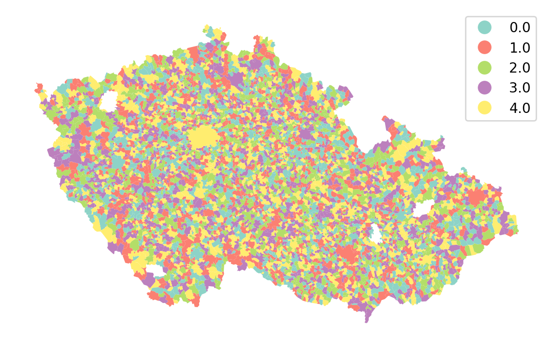
Allocation of polygons to k folds under random sampling

Spatial cross-validation mitigates the issue by including a spatial dimension in the train-test split. The aim is to divide the whole study area into smaller regions and allocate whole regions to train and test splits. You can do that based on many criteria, but it is handy to have a variable representing those regions as the "okres" column in your DataFrame.

Instead of using KFold, use GroupKFold, which ensures that observations are allocated into splits by groups (all observations within a single group will be in a single split).

gkf = model_selection.GroupKFold(n_splits=5)

Generate the same visualisation as above, with one difference - specifying the groups.

splits = gkf.split(
    independent,
1    groups=executions_data["okres"],
)
split_label = np.empty(len(independent), dtype=float)
for i, (train, test) in enumerate(splits):
    split_label[test] = i

executions_data.plot(
    split_label, categorical=True, legend=True, cmap="Set3"
).set_axis_off()

1: Use the "okres" column as an indication of groups that shall not be broken.

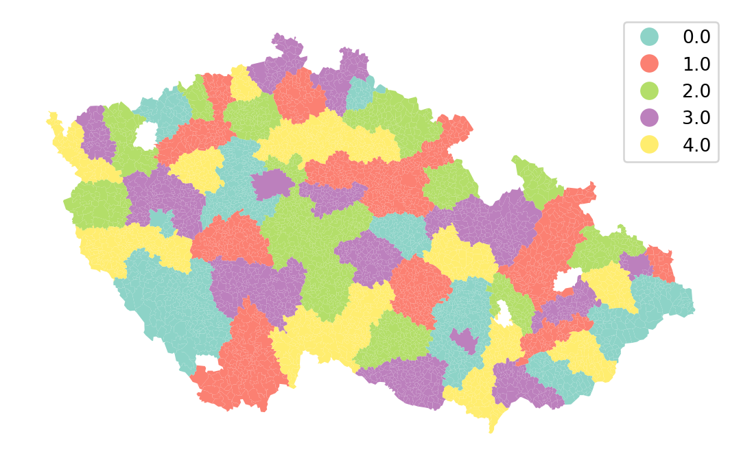
Allocation of polygons to k folds under spatial sampling

Cross-validated prediction can then be performed using these splits, ensuring that the spatial leakage between test and train is limited in each fold.

rf_spatial_cv = ensemble.RandomForestRegressor(random_state=0, n_jobs=-1)

pred_spatial_cv = model_selection.cross_val_predict(
    rf_spatial_cv,
    independent,
    target,
1    groups=executions_data["okres"],
2    cv=gkf,
    n_jobs=-1,
)

1: Pass the group labels.
2: And the GroupKFold object to cross_val_predict to make use of it.

The rest can follow the same pattern.

r2_spatial_cv = metrics.r2_score(target, pred_spatial_cv)
mae_spatial_cv = metrics.mean_absolute_error(target, pred_spatial_cv)
rmse_spatial_cv = metrics.root_mean_squared_error(target, pred_spatial_cv)

summary += f"""\
Random Forest with spatial cross-validation (k-fold):
  R2:   {round(r2_spatial_cv, 3)}
  MAE:  {round(mae_spatial_cv, 3)}
  RMSE: {round(rmse_spatial_cv, 3)}
"""
print(summary)

Evaluation metrics
==================
Random Forest:
  R2:   0.559
  MAE:  1.661
  RMSE: 2.555
Random Forest (k-fold metrics):
  R2:   0.527
  MAE:  1.695
  RMSE: 2.62
Random Forest with spatial cross-validation (k-fold):
  R2:   0.545
  MAE:  1.671
  RMSE: 2.569

The models with spatial cross-validation usually show worse performance than those with the random one but that is expected. The difference is due to elimination of the spatial leakage and hence improving the robustness of the model, meaning that on unseen data, it will perform better (contrary to the change in the metrics).

Model comparison

Now that you know how to embed geography in train-test splits and in the model evaluation, let’s have a look at some other models than Random Forest.

The API of them all will be mostly the same but note that some (like support vector regressor for example), may need data standardisation. For a comparison, check the performance of out-of-the-shelf Gradient Boosted Tree on our data using the spatial cross-validation.

boosted_tree = ensemble.GradientBoostingRegressor()
pred_boosted_tree = model_selection.cross_val_predict(
    boosted_tree,
    independent,
    target,
    groups=executions_data.okres,
    cv=gkf,
)

r2_boosted_tree = metrics.r2_score(target, pred_boosted_tree)
mae_boosted_tree = metrics.mean_absolute_error(target, pred_boosted_tree)
rmse_boosted_tree = metrics.root_mean_squared_error(target, pred_boosted_tree)

summary += f"""\
Gradient Boosted Tree with spatial cross-validation (k-fold):
  R2:   {round(r2_boosted_tree, 3)}
  MAE:  {round(mae_boosted_tree, 3)}
  RMSE: {round(rmse_boosted_tree, 3)}
"""
print(summary)

Evaluation metrics
==================
Random Forest:
  R2:   0.559
  MAE:  1.661
  RMSE: 2.555
Random Forest (k-fold metrics):
  R2:   0.527
  MAE:  1.695
  RMSE: 2.62
Random Forest with spatial cross-validation (k-fold):
  R2:   0.545
  MAE:  1.671
  RMSE: 2.569
Gradient Boosted Tree with spatial cross-validation (k-fold):
  R2:   0.557
  MAE:  1.652
  RMSE: 2.536

As you can see, the gradient boosted tree over-performs the random forest model. However, using the default parameters may not yield the optimal model.

Hyper-parameter tuning

When searching for an optimal model, you shall test different hyper-parameters. Let’s stick to the gradient boosted tree for now and test the performance of a sequence of models comparing different way of measuring the loss and different learning rates.

1param_grid = {
    "loss": ["squared_error", "absolute_error"],
    "learning_rate": [0.01, 0.05, 0.1, 0.15, 0.2],
}

2boosted_tree = ensemble.GradientBoostingRegressor(random_state=0)

3grid_search = model_selection.GridSearchCV(
    boosted_tree, param_grid, cv=gkf
)
4grid_search.fit(independent, target, groups=executions_data.okres)

1: Specify the parameters for a grid search. Since we have two dimensions here (loss and learning rate), the grid will test 2x5 models and compare them all.
2: Define a fresh model.
3: Define a grid search. Pass in the information on the spatial split to make use of it.
4: Fit the data. This fits all 10 models and measures their performance using the default scorer.

GridSearchCV(cv=GroupKFold(n_splits=5),
             estimator=GradientBoostingRegressor(random_state=0),
             param_grid={'learning_rate': [0.01, 0.05, 0.1, 0.15, 0.2],
                         'loss': ['squared_error', 'absolute_error']})

Large grid searches may take a while as there’s often a lot of models to train. The result contains many pieces of information, from score and parameters to time required to train each model.

Let’s extract the mean test scores per each model and figure out which parameters are the best in this case.

1params = grid_search.cv_results_["params"]
2mean_scores = grid_search.cv_results_["mean_test_score"]

3grid_search_results = pd.DataFrame(params)
grid_search_results["mean_score"] = mean_scores
grid_search_results.sort_values("mean_score", ascending=False)

1: Extract parameters of each model.
2: And the mean test score.
3: Get it all into a single DataFrame.

	learning_rate	loss	mean_score
7	0.15	absolute_error	0.554728
5	0.10	absolute_error	0.552654
9	0.20	absolute_error	0.545557
4	0.10	squared_error	0.545254
2	0.05	squared_error	0.544545
3	0.05	absolute_error	0.538022
6	0.15	squared_error	0.537972
8	0.20	squared_error	0.533400
0	0.01	squared_error	0.404032
1	0.01	absolute_error	0.277876

The best model seems to be use learning rate of 0.15 and absolute error as a measure of loss. The score here is \(R^2\), so you may wonder how come it is smaller than before? It is a mean of 5 folds, not a single score derived from cross-validated prediction, hence the number has slightly different properties. Remember, \(R^2\), while being usually in the same ballpark range, is not directly comparable across datasets.

Feature importance

There is one more question you may ask. What is driving the results?

Get the best model from the grid search and explore the importance of individual independent variables.

best_model = grid_search.best_estimator_

Feature importance is not directly comparable to \(\beta\) coefficients. The values sum to 1 and indicate the normalised reduction of the loss brought by each feature. The higher the value, the more important the feature is within the model.

1feature_importance = pd.Series(
    best_model.feature_importances_, index=independent_variables
)
feature_importance.sort_values()

1: Extract feature importance and wrap them into a Series indexed by variable names for easier interpretation.

mean_age             0.031129
masters_degree       0.046091
AndrejBabis          0.103890
primary_education    0.147787
divorced             0.326221
undetermined         0.344883
dtype: float64

Two out of the six independent variables account for mode than 66% of the model performance. Let’s see that visually.

feature_importance.sort_values(ascending=False).plot.bar()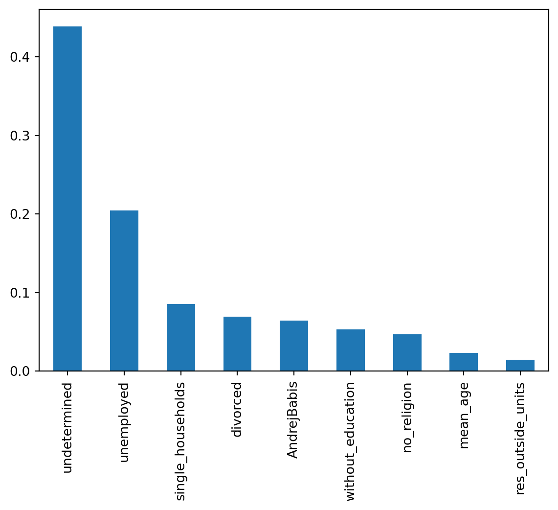

The rate of divorces playing a role is a bit expected. What is really interesting is that the most important variable is the proportion of population with undetermined education level. While many other types of information are coming from various national registries, the education is likely dependent on the information provided during the Census. And it seems, that people who struggle with executions do not trust the government enough, to provide such a basic data.

You can compare the original baseline model with the “best” one spatially or try to get a Random Forest that outperforms this Gradient Boosted Tree. There is a lot to play with.

Additional reading

This material has intentionally omitted a lot of ML basics. Go and check the User Guide of scikit-learn to catch up with it yourself.