Population as a raster grid

Until now, all the data you were working with were tables. However, not everything is a table. Raster data are not that common in social geography, but spatial data science is full of it, from satellite imagery to population grids. In this session, you will learn how to work with spatial raster data in Python and how to link raster to vector using the ecosystem around the xarray package.

Arrays and their many dimensions

Raster data are represented as arrays. Those can take many forms and shapes. You already know pandas data structures, so let’s start with those.

A pandas.Series is a 1-dimensional array with an index. A typical array contains values of the same data type (e.g. float numbers), as does a typical Series.

When it comes to geospatial raster data, one dimension is not enough. Even the most basic raster, something like a digital terrain model (DTM), requires two dimensions. One represents longitude (or x when projected), while the other latitude (or y), resulting in a 2-dimensional array.

But you don’t have to stop there. Take a typical satellite image. The longitude and latitude dimensions are still present, but you have different bands representing blue, green, red and often near-infra-red frequencies, resulting in a 3-dimensional array (lon, lat, band). Throw in time, and you’re now dealing with a 4-dimensional array (lon, lat, band, time).

All these use cases fall under the umbrella of N-dimensional array handling covered by the xarray package. Whereas a pandas.Series is a 1-dimensional array with an index, xarray.DataArray is an N-dimensional array with N indexes. Combining multiple Series gives you a pandas.DataFrame, where each column can have a different data type (e.g. one numbers, other names). Combining multiple xarray.DataArrays gives you a xarray.Dataset, where each array can have a different data type. There’s a lot of similarity between pandas and xarray, but also some differences.

Let’s read some raster and explore xarray objects in practice.

import datashader as ds
import geopandas as gpd
import rioxarray
import xarray as xr
import osmnx as ox
import pandas as pd
import matplotlib.pyplot as plt
import xvec

Population grids

Today, you will be working with the data from the Global Human Settlement Layer (GHSL) developed by the Joint Research Centre of the European Commission. Unlike in all previous hands-on sessions, the data is not pre-processed and you could read it directly from the open data repository. However, since that seems to be a bit unstable lately, use the copy stored as part of this course.

The first layer you will open is a population grid. GHSL covers the whole world divided into a set of tiles, each covering an area of 1,000 by 1,000 km at a resolution of 100m per pixel. The link below points to a single tile¹ covering most of Eastern Europe.

1pop_url = (
    "https://martinfleischmann.net/sds/raster_data/data/"
    "GHS_POP_E2030_GLOBE_R2023A_54009_100_V1_0_R4_C20.zip"
      )
pop_url

1: The URL is long. It may be better to write it as a multi-line string to avoid a long line.

'https://martinfleischmann.net/sds/raster_data/data/GHS_POP_E2030_GLOBE_R2023A_54009_100_V1_0_R4_C20.zip'

Original data

You can, alternatively, try reading the original data directly using this URL:

pop_url = (
    "https://jeodpp.jrc.ec.europa.eu/ftp/jrc-opendata/GHSL/"
    "GHS_POP_GLOBE_R2023A/GHS_POP_E2030_GLOBE_R2023A_54009_100/"
    "V1-0/tiles/GHS_POP_E2030_GLOBE_R2023A_54009_100_V1_0_R4_C20.zip"
      )

The pop_url points to a ZIP file. Within that ZIP file is a GeoTIFF containing the actual raster. There is often no need to download and unzip the file as there’s a good chance you can read it directly.

Reading rasters with `rioxarray`

xarray, like pandas is an agnostic library. It is designed for N-dimensional arrays but not necessarily geospatial arrays (although that is often the case…). It means that by default, it is not able to read geospatial file formats like GeoTIFF. That is where rioxarray comes in. It comes with the support of the usual geo-specific things like specific file formats or CRS.

1p = f"zip+{pop_url}!GHS_POP_E2030_GLOBE_R2023A_54009_100_V1_0_R4_C20.tif"
2population = rioxarray.open_rasterio(p, masked=True)
population

1: Create a path to the file inside the ZIP. Add the "zip+" prefix and then the path to the actual file inside the archive, starting with "!".
2: Use rioxarray to open the file using the lower-level rasterio package. With masked=True ensure, that the missing values are properly masked out.

Above, you can see the representation of the population grid as a DataArray. It has three dimensions ("band", "x", "y") with a resolution 1x10,000x10,000 and values as float.

rioxarray gives you a handy .rio accessor on xarray objects, allowing you to access geospatial-specific tools. Like retrieval of CRS.

population.rio.crs

CRS.from_wkt('PROJCS["World_Mollweide",GEOGCS["WGS 84",DATUM["WGS_1984",SPHEROID["WGS 84",6378137,298.257223563,AUTHORITY["EPSG","7030"]],AUTHORITY["EPSG","6326"]],PRIMEM["Greenwich",0],UNIT["Degree",0.0174532925199433]],PROJECTION["Mollweide"],PARAMETER["central_meridian",0],PARAMETER["false_easting",0],PARAMETER["false_northing",0],UNIT["metre",1,AUTHORITY["EPSG","9001"]],AXIS["Easting",EAST],AXIS["Northing",NORTH]]')

Or the extent of the raster (in the CRS shown above).

population.rio.bounds()

(959000.0, 5000000.0, 1959000.0, 6000000.0)

The missing, masked data can be represented as as specific value, especially when dealing with integer arrays. You can check which one:

population.rio.nodata

nan

Plotting with `datashader`

Plotting a raster with a resolution of 10,000x10,000 pixels can be tricky. Often, the resolution is even larger than that. The best way to plot is to resample the data to a smaller resolution that better fits the screen. A handy tool that can do that quickly is datashader. Let’s use it to plot the array as 600x600 pixels.

1canvas = ds.Canvas(plot_width=600, plot_height=600)
2agg = canvas.raster(population.where(population>0).sel(band=1))
agg

1: Create a canvas with a specific resolution.
2: Select pixels with a population more than 0 (population.where(population>0)), select a single band to get 2-dimensional array (.sel(band=1)) and pass the result to the canvas.

You can see that the result is a new xarray.DataArray with a resolution 600x600. The built-in matplotlib-based plotting can easily handle that.

_ = agg.plot()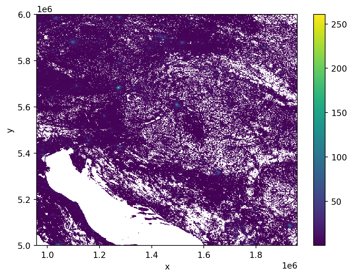

Population grid resampled to 600x600 pixels

Clipping based on geometry

Daling with large rasters is often impractical if you are interested in a small subset, for example, representing a single city.

Functional Urban Areas

In this case, you may want to work only with the data covering Budapest, Hungary, defined by its functional urban area (FUA), available as another data product on GHSL. FUAs are available as a single GeoPackage with vector geometries.

1fua_url = (
    "https://martinfleischmann.net/sds/raster_data/data/"
    "GHS_FUA_UCDB2015_GLOBE_R2019A_54009_1K_V1_0.zip"
)
2p = f"zip+{fua_url}!GHS_FUA_UCDB2015_GLOBE_R2019A_54009_1K_V1_0.gpkg"
3fuas = gpd.read_file(p)
4budapest = fuas.query("eFUA_name == 'Budapest'")
budapest.explore()

1: Get the URL.
2: Specify the path to read the file from the ZIP.
3: Read the table with geopandas.
4: Filter only Budapest.

Make this Notebook Trusted to load map: File -> Trust Notebook

Original data

You can, alternatively, try reading the original data directly using this URL:

fua_url = (
    "https://jeodpp.jrc.ec.europa.eu/ftp/jrc-opendata/GHSL/"
    "GHS_FUA_UCDB2015_GLOBE_R2019A/V1-0/"
    "GHS_FUA_UCDB2015_GLOBE_R2019A_54009_1K_V1_0.zip"
)

If you want to clip the population raster to the extent of Budapest FUA, you can use the clip method from the rioxarray extension of xarray.

1population_bud = population.rio.clip(
2    budapest.to_crs(population.rio.crs).geometry
)
population_bud

1: Use .rio.clip to clip the geospatial raster to the extent of a geometry.
2: Ensure the budapest is in the same CRS as the population and pass its geometry.

The raster is no longer 10,000x10,000 pixels but only 840x830, covering the extent of Budapest FUA. You can easily check that by plotting the clipped array.

_ = population_bud.plot()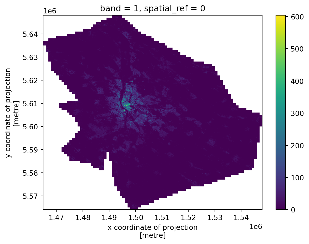

Array manipulation

While this is technically a 3-dimensional array, the dimension "band" has only one value. Normally, you would get a 2-dimensional array representing a selected band using the .sel() method.

population_bud.sel(band=1)

But if you have only one band, you can squeeze the array and get rid of that dimension that is not needed.

population_bud = population_bud.drop_vars("band").squeeze()
population_bud

Now a lot what you know from pandas works equally in xarray. Getting the minimum:

population_bud.min()

<xarray.DataArray ()> Size: 8B
array(0.)
Coordinates:
    spatial_ref  int64 8B 0

As expected, there are some cells with no inhabitants.

population_bud.max()

<xarray.DataArray ()> Size: 8B
array(603.90405273)
Coordinates:
    spatial_ref  int64 8B 0

The densest cell, on the other hand, has more than 600 people per hectare.

population_bud.mean()

<xarray.DataArray ()> Size: 8B
array(6.77593517)
Coordinates:
    spatial_ref  int64 8B 0

Mean is, however, only below 7.

population_bud.median()

<xarray.DataArray ()> Size: 8B
array(0.)
Coordinates:
    spatial_ref  int64 8B 0

While the median is 0, there are a lot of cells with 0.

DataArray vs scalar

Notice that xarray always returns another DataArray even with a single value. If you want to get that scalar value, you can use .item().

population_bud.mean().item()

6.775935172506021

You can plot the distribution of values across the array.

_ = population_bud.plot.hist(bins=100)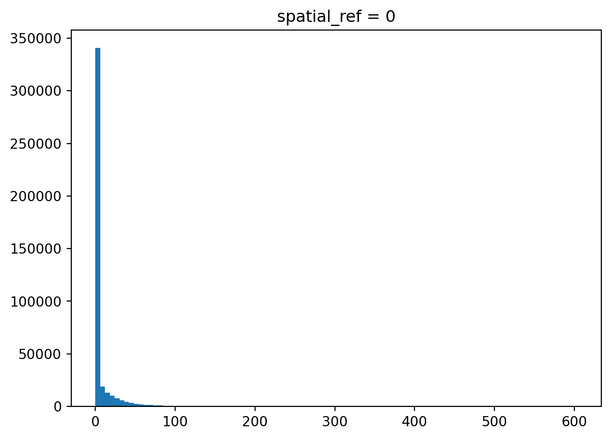

Indeed, there are a lot of zeros. Let’s filter them out and check the distribution again.

_ = population_bud.where(population_bud>0).plot.hist(bins=100)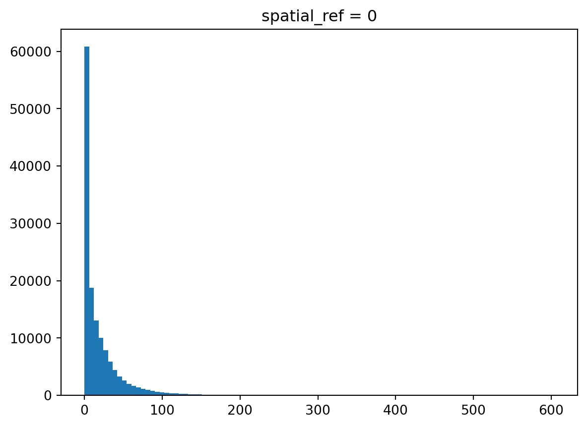

Histogram of population counts excluding 0

As with many observations in urban areas, this follows a power-law-like distribution with a lot of observations with tiny values and only a few with large ones.

Array operations

Let’s assume that you want to normalise population counts by the built-up volume, which is available as another GHSL product. This time, on a grid again.

volume_url = (
    "https://martinfleischmann.net/sds/raster_data/data/"
    "GHS_BUILT_V_E2030_GLOBE_R2023A_54009_100_V1_0_R4_C20.zip"
)
volume_url

'https://martinfleischmann.net/sds/raster_data/data/GHS_BUILT_V_E2030_GLOBE_R2023A_54009_100_V1_0_R4_C20.zip'

Backup data

You can, alternatively, try reading the original data directly using this URL:

volume_url = (
    "https://jeodpp.jrc.ec.europa.eu/ftp/jrc-opendata/GHSL/"
    "GHS_BUILT_V_GLOBE_R2023A/GHS_BUILT_V_E2030_GLOBE_R2023A_54009_100/V1-0/tiles/"
    "GHS_BUILT_V_E2030_GLOBE_R2023A_54009_100_V1_0_R4_C20.zip"
)

All work the same as before. You read the GeoTIFF as a DataArray.

p = f"zip+{volume_url}!GHS_BUILT_V_E2030_GLOBE_R2023A_54009_100_V1_0_R4_C20.tif"
built_up = rioxarray.open_rasterio(p, masked=True).drop_vars("band").squeeze()
built_up

And clip it to the same extent.

built_up_bud = built_up.rio.clip(budapest.to_crs(built_up.rio.crs).geometry)
built_up_bud

You can quickly check what it looks like.

_ = built_up_bud.plot(cmap="magma_r")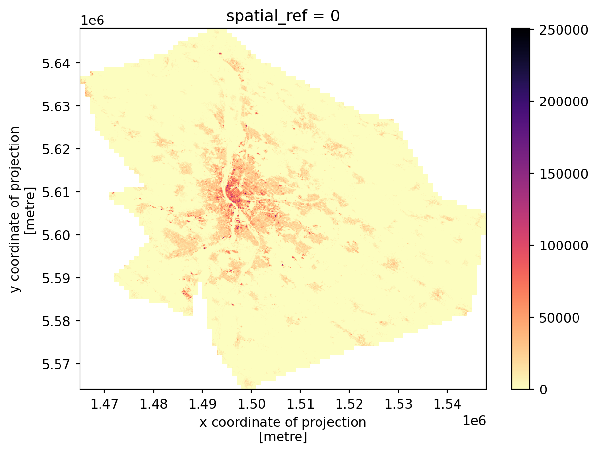

The two grids are aligned, meaning that pixels with the same coordinates represent the same area. This allows us to directly perform array algebra. Again, you know this from pandas.

1pop_density = population_bud /  built_up_bud
pop_density

1: Divide the population by built-up volume to get a normalised value.

The result is a new array that inherits spatial information (spatial_ref) but contains newly computed values.

_ = pop_density.plot(cmap="cividis_r")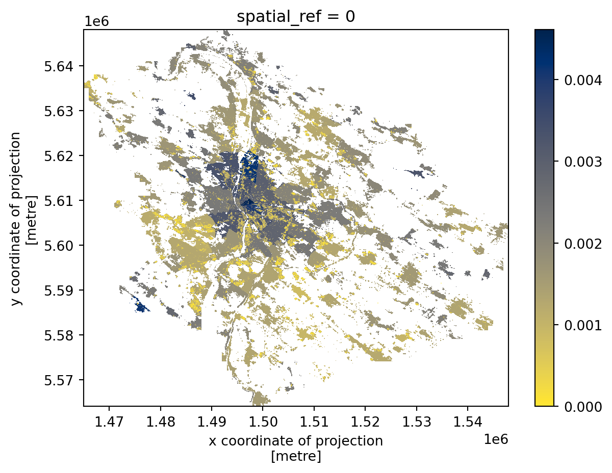

Population grid normalised by the built-up volume

The resulting array can then be saved to a GeoTIFF using rioxarray.

pop_density.rio.to_raster("population_density.tif")

Extracting values for locations

A common need is to extract values from raster data for a specific location of interest. That is a first type of interaction between raster and vector data (points in this case). To illustrate the use case, create a set of random points covering the area of budapest.

1locations = budapest.sample_points(1000).explode(ignore_index=True)
locations.head()

1: sample_points() method creates a random sample of the selected size within each geometry in a GeoSeries. Each sample set is a MultiPoint but in this case, you want individual points. That is when explode() is useful, since it explodes each multi-part geometry into individual points. Because you are not interested in the original index, you can use ignore_index=True to get the default pd.RangeIndex.

0    POINT (1465434.374 5635035.186)
1    POINT (1465649.409 5635673.247)
2    POINT (1466040.233 5635649.787)
3    POINT (1466348.314 5635038.692)
4    POINT (1467546.109 5632642.335)
Name: sampled_points, dtype: geometry

Check how the sample looks on a map.

locations.explore()

Make this Notebook Trusted to load map: File -> Trust Notebook

Random sampling and reproducibility

The points sampled from budapest will be different every time you run the sample_points() method. If you want to fix the result, you can pass a seed value to a random number generator as rng=42. With the same seed value, the result will be always the same. This is useful, especially if you are interested in the reproducibility of your code.

The xarray ecosystem offers many ways of extracting point values. Below, you will use the implementation from the xvec package. Create a new xarray.DataArray with all three arrays you created so far to see the benefits of using xvec below.

1bud_cube = xr.concat(
2    [pop_density, population_bud, built_up_bud],
3    dim=pd.Index(
4        ["density", "population", "built-up volume"],
5        name="measurement",
    )
)
bud_cube

1: Use xr.concat function to concatenate all arrays together.
2: Specify which arrays shall be concatenated.
3: Define a new dimension created along the axis of concatenation. Use the pd.Index to create a new index along this dimension.
4: Specify coordinates along the new dimension.
5: Give the dimension a name.

The resulting DataArray is 3-dimensional, compared to 2-dimensional arrays used before. Apart from x and y, you now have measurement as well. Using the new index created above, you can use the sel() method to get the original arrays.

bud_cube.sel(measurement="density")

Now it is time to take this cube and create another based on your points. That can be done using the .xvec accessor and its extract_points method.

1vector_cube = bud_cube.drop_vars("spatial_ref").xvec.extract_points(
2    points=locations.geometry,
3    x_coords="x",
    y_coords="y",
)
vector_cube

1: Drop spatial_ref because it is not interesting for point extraction and use .xvec.extract_points()
2: Specify the points for which you want to extract the values.
3: Specify which dimension of the bud_cube DataArray represents x-coordinate dimension of geometries and which represents the y-coordinate dimension to match points to the array.

The resulting object is still a DataArray but a bit different. It is no longer 3-dimensional, although all dimensions of interest ('density', 'population', 'built-up volume') are still there, but 2-dimensional. One dimension is measurement, and the other is geometry, containing the points of interest. With xvec, the spatial dimension is reduced, but the remaining dimensionality of the original array is preserved.

You can then convert the data into a geopandas.GeoDataFrame and work with it as usual.

location_data = vector_cube.xvec.to_geopandas()
location_data.head()

measurement	geometry	density	population	built-up volume
0	POINT (1465434.374 5635035.186)	0.001112	22.687181	20399.0
1	POINT (1465649.409 5635673.247)	0.001040	18.316349	17605.0
2	POINT (1466040.233 5635649.787)	0.000850	3.800289	4470.0
3	POINT (1466348.314 5635038.692)	0.001112	9.474587	8519.0
4	POINT (1467546.109 5632642.335)	0.001112	5.907854	5312.0

Check the result on a map to verify that all worked as expected.

location_data.explore("density", cmap="cividis_r", tiles="CartoDB Positron")

Make this Notebook Trusted to load map: File -> Trust Notebook

Vector data cubes

The data structure vector_cube represents is called a vector data cube. It is a special case of an xarray N-dimensional object, where at least one dimension is indexed by geometries. See more in the Xvec documentation.

Zonal statistics

Another operation when working with rasters is the transfer of values from an array to a set of polygons. This is called zonal statistics and can be done in many ways, depending on the use case. In most cases, one of the methods available in xvec should cover your specific needs.

Downloading OpenStreetMap data

You may be interested in the average population density in individual districts of Budapest. One option for getting the geometries representing the districts is the OpenStreetMap. Everything you can see on OpenStreetMap is downloadable. In Python, a recommended way (when not doing large downloads) is the osmnx package (imported as ox). The detailed explanation of osmnx is out of scope for this session, but if you are interested in details, check the official Getting started guide.

1admin_level_9 = ox.features_from_place("Budapest", {"admin_level": "9"})
2districts = admin_level_9[admin_level_9.geom_type == "Polygon"][
3    ["name", "name:en", "geometry"]
]
4districts["key"] = range(len(districts))
5districts = districts.to_crs(pop_density.rio.crs)

1: Use features_from_place to download features from Budapest. But filter only those tagged with the admin_level equal to 9.
2: Filter only polygons. The GeoDataFrame coming from osmnx also contains many LineStrings.
3: Retain only three columns that may be useful.
4: Create a new column with a key - an integer value unique to each observation. That will be useful later.
5: Ensure the geometry uses the same CRS as the grid.

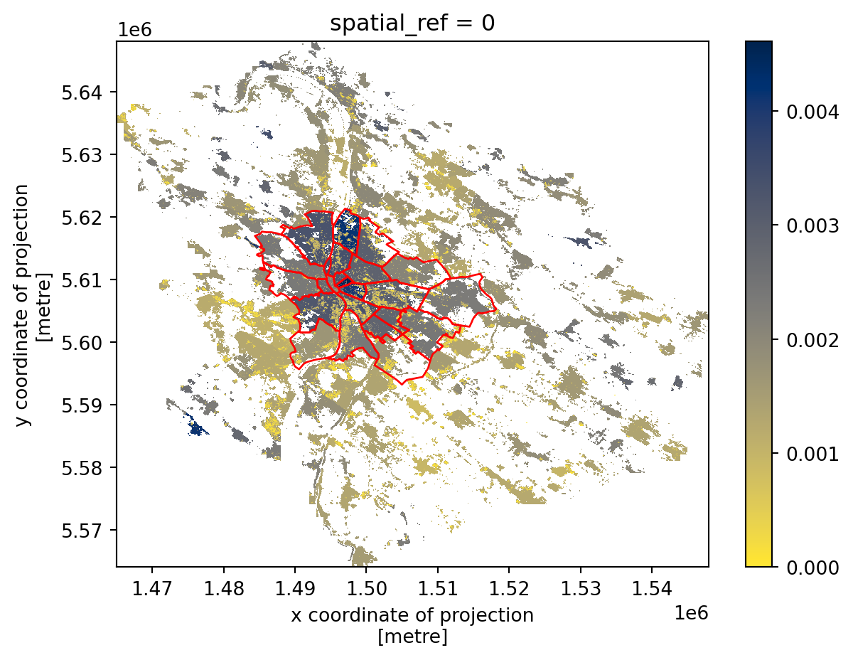
Plotting raster and vector together

Both xarray and geopandas can create matplotlib plots that can be combined to see how the two overlap.

1f, ax = plt.subplots()
2pop_density.plot(ax=ax, cmap="cividis_r")
3districts.plot(
4    ax=ax, facecolor="none", edgecolor="red", linewidth=1, aspect=None
);

1: Create an empty figure and an axis.
2: Plot the population density to the axis.
3: Plot the districts to the same array, ensuring it is in the same projection.
4: Specify the plotting style and disable the automatic setting of the aspect to keep the axis as returned by xarray.

Overlay of district boundaries over population density

Zonal statistics

Zonal statistics using xvec is as simple as point data extraction, with the only difference that you can optionally specify the type of aggregation you’d like to extract. By default, you get mean.

1zonal_stats = bud_cube.drop_vars("spatial_ref").xvec.zonal_stats(
2    geometry=districts.geometry,
3    x_coords="x",
    y_coords="y",
)
zonal_stats

1: Drop spatial_ref because it is not interesting for point extraction and use .xvec.zonal_stats()
2: Specify the geometries for which you want to aggregate the values.
3: Specify which dimension of the bud_cube DataArray represents x-coordinate dimension of geometries and which represents the y-coordinate dimension to match geometries to the array.

The result is again a vector data cube. Though mean is not the optimal aggregation method for population. Let’s refine the code above a bit to get more useful aggregation.

zonal_stats = bud_cube.drop_vars("spatial_ref").xvec.zonal_stats(
    geometry=districts.geometry,
    x_coords="x",
    y_coords="y",
3    stats=["mean", "sum", "median", "min", "max"],
)
zonal_stats

3: Specify which aggregations should xvec return as a list.

You may have noticed that our data cube now has one more dimension zonal_statistics, reflecting each of the aggregation methods specified above.

Other statistics

The stats keyword is quite flexible and allows you to pass even your custom functions. Check the documentation for details.

To check the result on a map, convert the data to a geopandas.GeoDataFrame again.

zones = zonal_stats.xvec.to_geodataframe(name="stats")
zones

		geometry	index	stats
zonal_statistics	measurement
mean	density	POLYGON ((1494534.328 5597452.839, 1494709.464...	(relation, 215618)	0.001935
	population	POLYGON ((1494534.328 5597452.839, 1494709.464...	(relation, 215618)	30.551469
	built-up volume	POLYGON ((1494534.328 5597452.839, 1494709.464...	(relation, 215618)	19338.583016
sum	density	POLYGON ((1494534.328 5597452.839, 1494709.464...	(relation, 215618)	4.327341
sum	population	POLYGON ((1494534.328 5597452.839, 1494709.464...	(relation, 215618)	80228.156869
...	...	...	...	...
min	population	POLYGON ((1494292.33 5610780.086, 1494393.558 ...	(relation, 1606103)	0.000000
min	built-up volume	POLYGON ((1494292.33 5610780.086, 1494393.558 ...	(relation, 1606103)	0.000000
max	density	POLYGON ((1494292.33 5610780.086, 1494393.558 ...	(relation, 1606103)	0.004608
	population	POLYGON ((1494292.33 5610780.086, 1494393.558 ...	(relation, 1606103)	344.663391
	built-up volume	POLYGON ((1494292.33 5610780.086, 1494393.558 ...	(relation, 1606103)	115273.000000

345 rows × 3 columns

Check the result on a map to verify that all worked as expected. Get mean density and explore its values, stored in the stats column.

zones.loc[("mean", 'density')].explore("stats", cmap="cividis_r", tiles="CartoDB Positron")

/tmp/ipykernel_4219/4164103204.py:1: PerformanceWarning: indexing past lexsort depth may impact performance.
  zones.loc[("mean", 'density')].explore("stats", cmap="cividis_r", tiles="CartoDB Positron")

Make this Notebook Trusted to load map: File -> Trust Notebook

Additional reading

Have a look at the chapter Local Spatial Autocorrelation from the Geographic Data Science with Python by Rey, Arribas-Bel, and Wolf (2023) to learn how to do LISA on rasters.

The great resource on xarray is their tutorial.

References

Rey, Sergio, Dani Arribas-Bel, and Levi John Wolf. 2023. Geographic Data Science with Python. Chapman & Hall/CRC Texts in Statistical Science. London, England: Taylor & Francis.

Footnotes

See the distribution of tiles in the data repository.↩︎

Arrays and their many dimensions

Population grids

Reading rasters with rioxarray

Plotting with datashader

Clipping based on geometry

Functional Urban Areas

Array manipulation

Array operations

Extracting values for locations

Zonal statistics

Downloading OpenStreetMap data

Plotting raster and vector together

Zonal statistics

References

Footnotes

Reading rasters with `rioxarray`

Plotting with `datashader`