1import geopandas as gpd
import shapely- 1
-
As you import
pandasaspd, you can importgeopandasasgpdto keep things shorter.
It is time to get your hands on some spatial data. You will not go far from your pandas experience, you’ll just expand it a bit. This section covers an introduction to geopandas, a Python package extending the capabilities of pandas by providing support for geometries, projections and geospatial file formats. Let’s start with importing geopandas.
1import geopandas as gpd
import shapelypandas as pd, you can import geopandas as gpd to keep things shorter.
You will be using a few different datasets in this notebook. The first one contains data on buildings, streets and street junctions of a small part of Paris from Fleischmann et al. (2021). The data contain some information on urban morphology derived from these geometries, but today, you will be mostly interested in geometries, not so much in attributes.
Assuming you have a file containing both data and geometry (e.g. GeoPackage, GeoJSON, Shapefile), you can read it using geopandas.read_file(), which automatically detects the file type and creates a geopandas.GeoDataFrame. A geopandas.GeoDataFrame is just like pandas.DataFrame but with additional column(s) containing geometry (in simple terms).
"buildings", you need to pass layer="buildings". Otherwise, geopandas will read the first available layer.
| uID | blg_area | wall | adjacency | neighbour_distance | nID | length | linearity | width | width_deviation | openness | mm_len | node_start | node_end | nodeID | meshedness | geometry | |
|---|---|---|---|---|---|---|---|---|---|---|---|---|---|---|---|---|---|
| 0 | 0 | 27194.254623 | 1079.492255 | 0.423913 | 79.492252 | 1 | 238.865434 | 0.999987 | 50.00000 | 0.000000 | 1.00000 | 238.865434 | 1 | 5 | 5 | 0.153846 | POLYGON ((449483.67 5412864.072, 449488.881 54... |
| 1 | 1 | 2196.125585 | 255.198183 | 0.857143 | 52.080293 | 17 | 213.373518 | 0.999935 | 40.47981 | 0.580373 | 0.78169 | 213.373518 | 7 | 84 | 7 | 0.163934 | POLYGON ((449751.333 5412374.461, 449752.33 54... |
| 2 | 2 | 34.882075 | 39.461749 | 0.583333 | 49.413639 | 17 | 213.373518 | 0.999935 | 40.47981 | 0.580373 | 0.78169 | 213.373518 | 7 | 84 | 84 | 0.209302 | POLYGON ((449714.614 5412302.731, 449714.577 5... |
| 3 | 3 | 38.808817 | 39.461749 | 0.600000 | 43.450128 | 17 | 213.373518 | 0.999935 | 40.47981 | 0.580373 | 0.78169 | 213.373518 | 7 | 84 | 84 | 0.209302 | POLYGON ((449712.682 5412306.562, 449702.048 5... |
| 4 | 4 | 90.426163 | 255.198183 | 0.833333 | 12.131337 | 17 | 213.373518 | 0.999935 | 40.47981 | 0.580373 | 0.78169 | 213.373518 | 7 | 84 | 84 | 0.209302 | POLYGON ((449725.342 5412337.375, 449720.863 5... |
You can quickly check which layers are available in the GPKG file using geopandas.list_layers().
gpd.list_layers(paris_url)| name | geometry_type | |
|---|---|---|
| 0 | tessellation | Unknown |
| 1 | buildings | Polygon |
| 2 | edges | LineString |
| 3 | nodes | Point |
Let’s have a quick look at the "geometry" column. This is the special one enabled by geopandas. You can notice that the objects stored in this column are not float or string but Polygons of a geometry data type instead. The column is also a geopandas.GeoSeries instead of a pandas.Series.
buildings["geometry"].head()0 POLYGON ((449483.67 5412864.072, 449488.881 54...
1 POLYGON ((449751.333 5412374.461, 449752.33 54...
2 POLYGON ((449714.614 5412302.731, 449714.577 5...
3 POLYGON ((449712.682 5412306.562, 449702.048 5...
4 POLYGON ((449725.342 5412337.375, 449720.863 5...
Name: geometry, dtype: geometryPolygons are not the only geometry types you can work with. The same GPKG that contains buildings data also includes street network geometries of a LineString geometry type.
1street_edges = gpd.read_file(paris_url, layer="edges")
street_edges.head(2)"edges".
| length | linearity | width | width_deviation | openness | mm_len | node_start | node_end | nID | geometry | |
|---|---|---|---|---|---|---|---|---|---|---|
| 0 | 35.841349 | 1.000000 | 50.0 | 0.0 | 1.0 | 35.841349 | 1 | 2 | 0 | LINESTRING (449667.399 5412675.189, 449666.378... |
| 1 | 238.865434 | 0.999987 | 50.0 | 0.0 | 1.0 | 238.865434 | 1 | 5 | 1 | LINESTRING (449687.083 5412913.239, 449683.137... |
You can also load another layer, this time with Point geometries representing street network junctions.
1street_nodes = gpd.read_file(paris_url, layer="nodes")
street_nodes.head(2)"nodes". But more on that later.
| meshedness | nodeID | geometry | |
|---|---|---|---|
| 0 | 0.168 | 1 | POINT (449667.399 5412675.189) |
| 1 | 0.160 | 2 | POINT (449664.238 5412639.488) |
To write a GeoDataFrame back to a file, use GeoDataFrame.to_file(). The file is format automatically inferred from the suffix, but you can specify your own with the driver= keyword. When no suffix is given, GeoPandas expects that you want to create a folder with an ESRI Shapefile.
buildings.to_file("buildings.geojson")Geometries within the geometry column are shapely objects. GeoPandas itself is not creating the object but leverages the existing ecosystem (note that there is a significant overlap of the team writing both packages to ensure synergy). A typical GeoDataFrame contains a single geometry column, as you know from traditional GIS software. If you read it from a file, it will most likely be called "geometry", but that is not always the case. Furthermore, a GeoDataFrame can contain multiple geometry columns (e.g., one with polygons, another with their centroids and another with bounding boxes), of which one is considered active. You can always get this active column, no matter its name, by using .geometry property.
buildings.geometry.head()0 POLYGON ((449483.67 5412864.072, 449488.881 54...
1 POLYGON ((449751.333 5412374.461, 449752.33 54...
2 POLYGON ((449714.614 5412302.731, 449714.577 5...
3 POLYGON ((449712.682 5412306.562, 449702.048 5...
4 POLYGON ((449725.342 5412337.375, 449720.863 5...
Name: geometry, dtype: geometryIn data frames, you can usually access a column via indexer (df["column_name"]) or a property (df.column_name). However, the property is not available when there is either a method (e.g. .plot) or a built-in property (e.g. .crs or .geometry) overriding this option.
You can quickly check that the geometry is a data type indeed coming from shapely. You will use shapely directly in some occasions but in most cases, any interaction with shapely will be handled by geopandas.
type(buildings.geometry.loc[0])shapely.geometry.polygon.PolygonThere is also a handy SVG representation if you are in a Jupyter Notebook.
buildings.geometry.loc[0]
If you’d rather see a text representation, you can retrieve a Well-Known Text using .wkt property.
buildings.geometry.loc[0].wkt'POLYGON ((449483.67042272736 5412864.072456881, 449488.88104846893 5412863.625060784, 449510.6982350738 5412861.748884251, 449510.82232527074 5412863.304151067, 449510.9970363802 5412863.969594091, 449511.66399917164 5412863.919089544, 449511.51741561835 5412863.119987088, 449511.4365228922 5412861.475392743, 449511.92777931073 5412861.459829652, 449511.847098327 5412860.649013683, 449514.8591315278 5412860.388296289, 449517.71725811594 5412860.140090327, 449517.7760377807 5412860.962221627, 449518.2373559536 5412860.880227586, 449518.4419134186 5412862.412532236, 449518.4869309123 5412863.334841713, 449519.14666073857 5412863.295520584, 449519.1506655881 5412862.117074884, 449519.0673703245 5412861.017238655, 449541.1115176094 5412859.094659338, 449545.97766938613 5412858.672666636, 449549.75438190147 5412901.605985229, 449547.6073362831 5412901.814392851, 449548.567713732 5412913.122884805, 449550.67869009526 5412912.981506093, 449550.8025672962 5412914.514541514, 449551.9241080391 5412914.448813682, 449551.9348595453 5412914.826696844, 449552.39014691365 5412914.889282009, 449552.7947021043 5412915.0190284075, 449553.1844895202 5412915.137791312, 449553.567345395 5412915.301085203, 449553.995208161 5412915.575142834, 449554.3717355797 5412915.8496647095, 449554.6825619913 5412916.158131939, 449554.9271848004 5412916.444963708, 449555.21068708715 5412916.976019454, 449555.4137206183 5412917.530037004, 449555.5064483717 5412918.051700801, 449555.5475392717 5412918.540480322, 449555.62429303036 5412918.917766655, 449555.70998869033 5412919.472845257, 449556.1422696238 5412919.424468057, 449556.2183238966 5412920.535487359, 449562.79918093735 5412919.9534816, 449562.68676143093 5412918.87614223, 449563.11170885165 5412918.827831876, 449563.098344999 5412918.160928504, 449563.126774911 5412918.0606178325, 449563.1995080086 5412917.993257815, 449563.4046481416 5412917.969168958, 449564.15418411116 5412918.129148356, 449564.8460561479 5412918.400819888, 449565.3473547241 5412918.685331517, 449565.7600469264 5412918.903941842, 449569.385767247 5412920.005104809, 449573.1341477573 5412920.882819934, 449576.0881864898 5412921.512024904, 449581.89650447795 5412922.282190066, 449587.2816820141 5412922.489214591, 449587.38605958334 5412924.300353636, 449591.37312920834 5412923.997514584, 449591.18928952987 5412921.508952306, 449591.41653090715 5412921.495781836, 449591.41823944415 5412920.873210528, 449596.2987062339 5412920.417780314, 449596.3557664515 5412921.050937689, 449596.6122418503 5412921.026386226, 449596.8473139128 5412923.5033686785, 449600.79761606036 5412923.189751511, 449600.6270395119 5412921.356976227, 449604.7781654215 5412920.541279472, 449608.5895365421 5412919.46184521, 449610.842163415 5412918.76335628, 449613.8387027025 5412917.602349282, 449616.76150549244 5412916.397541602, 449618.4267426552 5412915.6265414115, 449622.3539571713 5412913.56776845, 449623.31717624434 5412913.025450806, 449623.469776855 5412912.868433806, 449623.6237828398 5412912.867043071, 449623.7196217933 5412912.921762948, 449623.7717601848 5412913.010228663, 449623.8136481859 5412913.587937933, 449624.2902329334 5412913.572517156, 449624.38094090414 5412914.683404835, 449630.9178089899 5412914.101876877, 449630.8739143512 5412913.301844328, 449632.98429004755 5412913.093799805, 449632.85340290813 5412911.594177414, 449633.44139722886 5412911.733390482, 449633.3687635781 5412911.811865739, 449634.9688831225 5412913.576149886, 449636.64116364875 5412911.960194462, 449635.12241655105 5412910.272994659, 449634.22338476323 5412911.42616944, 449632.6486707013 5412910.8511823565, 449633.1723898306 5412908.745328067, 449633.6809331814 5412907.395571448, 449632.0965758859 5412906.564979016, 449632.24154219666 5412906.37467999, 449632.10109926015 5412906.253660282, 449632.1368641002 5412906.153283759, 449632.03248709446 5412905.965236017, 449632.0170169093 5412905.876439151, 449632.0597139131 5412905.731531769, 449633.3081509492 5412904.28615824, 449634.4403545097 5412902.964122151, 449634.68216361897 5412902.939704867, 449634.78533626033 5412902.994358722, 449634.90890402586 5412902.8709553685, 449635.0347800814 5412903.003223728, 449635.1948152892 5412902.857257005, 449636.31493905303 5412904.25901188, 449639.6449246257 5412902.661442981, 449640.48687111214 5412904.121295262, 449639.5787976075 5412905.085560614, 449641.6630449916 5412906.045047367, 449642.7772715006 5412904.356312055, 449640.7423521288 5412903.174038237, 449640.611049216 5412903.253043019, 449640.4141531476 5412902.565562294, 449641.946280098 5412902.4850290585, 449641.7802405506 5412900.340933944, 449642.58633828926 5412900.2669548765, 449641.96324695816 5412893.8024464715, 449640.8566696185 5412893.901372244, 449635.5822474328 5412832.038043762, 449638.0595410284 5412831.848923279, 449638.0408595018 5412831.404409284, 449640.52548717073 5412831.215223694, 449640.2731551761 5412828.449352107, 449641.3721107519 5412828.317144039, 449641.25518949685 5412826.739576128, 449642.9850470283 5412826.6239074115, 449642.7462798089 5412823.735625579, 449642.5234843125 5412820.9917214485, 449640.6764859113 5412821.130681849, 449640.60436957626 5412819.641646034, 449639.4024388879 5412819.741432611, 449639.2017432166 5412817.008446167, 449636.52673296514 5412817.232702173, 449636.31247223227 5412814.6221260065, 449636.0776919613 5412814.613128503, 449635.391206935 5412806.815145865, 449635.60368519445 5412806.790993489, 449635.31619423494 5412803.380649782, 449635.09618137043 5412803.382636058, 449634.4531948267 5412795.528675599, 449634.6365391388 5412795.527020349, 449634.33427926747 5412792.105693004, 449634.1290338704 5412792.118663054, 449633.46484657715 5412784.353830736, 449633.6555250439 5412784.352109246, 449633.4263937883 5412781.719433408, 449636.1014209998 5412781.495176044, 449635.8997192581 5412778.651028268, 449637.0362567257 5412778.618533815, 449636.91350504366 5412777.207774697, 449638.6796454757 5412777.047309087, 449638.4516202225 5412774.536910838, 449638.16603648325 5412771.337774179, 449636.4140600939 5412771.442526725, 449636.3054739868 5412769.9760544235, 449635.17044009484 5412770.175291397, 449634.93226927775 5412767.353707063, 449632.42581256223 5412767.565325888, 449632.42873048485 5412767.076148678, 449629.8196003863 5412767.288695651, 449624.6260454385 5412705.469124302, 449625.784097605 5412705.380848207, 449625.21140460705 5412698.815834385, 449624.397943989 5412698.889881964, 449624.2467621461 5412696.7678878335, 449622.6781100574 5412696.870988961, 449622.9853372693 5412695.96773253, 449623.03737723606 5412696.045082065, 449624.77562591207 5412694.41741188, 449623.2275823561 5412692.741596499, 449621.4324691968 5412694.569887813, 449622.5781581991 5412695.548960886, 449621.9609937083 5412697.055337553, 449619.946886898 5412696.562140484, 449618.43871866807 5412696.0532580735, 449617.65367872006 5412697.650087786, 449617.4612906789 5412697.462835124, 449617.3088849697 5412697.642084512, 449617.2127411392 5412697.554016263, 449617.09660338896 5412697.688469868, 449616.84715035616 5412697.679605605, 449615.4577352982 5412696.513744743, 449614.0239146523 5412695.3038170105, 449614.0138700707 5412695.003746988, 449614.07193893724 5412694.936520154, 449613.96102680376 5412694.837468275, 449614.05506242963 5412694.692097156, 449613.9148146695 5412694.593310224, 449615.29801661795 5412693.446877436, 449614.378878989 5412691.5652775355, 449613.7199415229 5412690.070425025, 449615.1281581061 5412689.257278229, 449616.2143748868 5412690.1479506185, 449617.32080266706 5412688.403696475, 449615.46040861116 5412687.064215939, 449614.2101139275 5412689.121047575, 449614.32072498364 5412689.186750986, 449613.7730910469 5412689.458506467, 449613.6485249513 5412687.847657164, 449611.4863254577 5412688.011707396, 449611.44292906555 5412687.267256037, 449604.8984623957 5412687.848871055, 449604.98897594935 5412688.937525766, 449604.5059418415 5412689.053059722, 449604.5606933101 5412689.43054534, 449604.5989694958 5412689.608072617, 449604.5414027555 5412689.73088034, 449604.3737269281 5412689.8435656335, 449604.19027872104 5412689.834105697, 449603.46974788094 5412689.640507303, 449602.6220300327 5412689.1701313285, 449600.81276603666 5412688.619505331, 449597.58413957 5412687.648137317, 449593.73212909856 5412686.682403454, 449590.3232660036 5412686.057297078, 449586.1306774322 5412685.550445473, 449580.3267357528 5412685.291617745, 449580.32784101204 5412684.602349706, 449576.2967979027 5412684.927825402, 449576.4195663769 5412686.338583104, 449570.9662473771 5412686.732503002, 449570.86578072567 5412685.354895004, 449566.86387329566 5412685.657880034, 449566.9359078913 5412686.324252794, 449564.6663129751 5412686.778335735, 449562.16364109446 5412687.412399851, 449560.02013056946 5412688.020983725, 449556.41506428015 5412689.220870763, 449553.900641493 5412690.177439789, 449551.7741126546 5412691.041565836, 449549.2033322462 5412692.254339157, 449546.7870676462 5412693.521301644, 449544.1300921956 5412694.934964047, 449543.9907479902 5412694.93622428, 449543.85049896775 5412694.837439101, 449543.77565188025 5412694.671360023, 449543.7859966721 5412694.1932326, 449543.08907447907 5412694.177301526, 449543.2259000398 5412693.086591521, 449536.6668787795 5412693.679535491, 449536.7721739575 5412694.779172678, 449536.2954700794 5412694.783484644, 449536.3540470338 5412695.583383606, 449536.34571388876 5412696.283834195, 449536.2855406757 5412696.929168368, 449536.174130714 5412697.586083068, 449535.95281281247 5412698.255109006, 449535.66327772563 5412698.680176544, 449535.1692984536 5412699.207147025, 449534.6375436876 5412699.6121715205, 449534.0386778037 5412699.8955154065, 449533.46090867126 5412700.078614915, 449533.49356261635 5412700.445182742, 449532.3722806281 5412700.544262435, 449532.5118394902 5412702.188325901, 449530.4231875316 5412702.373976488, 449531.3980906808 5412713.66009745, 449533.50090341247 5412713.418733721, 449537.16807661625 5412756.386379051, 449486.46780440013 5412760.725072889, 449486.34724242584 5412760.370418295, 449486.0722675962 5412759.972693572, 449485.6662904804 5412759.687325738, 449485.26855303056 5412759.501936954, 449484.7840175564 5412759.450738974, 449484.3823685349 5412759.64336604, 449483.67042272736 5412864.072456881))'But without an assigned coordinate reference system (CRS), you don’t know where this shape lies on Earth. Therefore, each geometry column has (optionally) assigned a CRS. That is always available via .crs.
buildings.crs<Projected CRS: EPSG:32631>
Name: WGS 84 / UTM zone 31N
Axis Info [cartesian]:
- E[east]: Easting (metre)
- N[north]: Northing (metre)
Area of Use:
- name: Between 0°E and 6°E, northern hemisphere between equator and 84°N, onshore and offshore. Algeria. Andorra. Belgium. Benin. Burkina Faso. Denmark - North Sea. France. Germany - North Sea. Ghana. Luxembourg. Mali. Netherlands. Niger. Nigeria. Norway. Spain. Togo. United Kingdom (UK) - North Sea.
- bounds: (0.0, 0.0, 6.0, 84.0)
Coordinate Operation:
- name: UTM zone 31N
- method: Transverse Mercator
Datum: World Geodetic System 1984 ensemble
- Ellipsoid: WGS 84
- Prime Meridian: GreenwichIf you check the type, you’ll notice it comes from the pyproj package. Note that you will likely never interact with that yourself.
type(buildings.crs)pyproj.crs.crs.CRSThe object with the CRS information has plenty of useful tricks. You can, for example, quickly check if it is a geographic (coordinates are latitude and longitude in degrees) or a projected CRS (x and y in meters, feet or similar).
buildings.crs.is_geographicFalsegeopandas is like a glue that brings different pieces of the Python ecosystem together. pandas for tabular data, shapely for geometries, pyogrio for interaction with GIS file formats or pyproj for CRS management.
Now you have a GeoDataFrame and can start working with its geometry.
Since there was only one geometry column in the buildings dataset, this column automatically becomes the active geometry and spatial methods used on the GeoDataFrame will be applied to the "geometry" column.
To measure the area of each polygon, access the GeoDataFrame.area attribute, which returns a pandas.Series. Note that GeoDataFrame.area is just GeoSeries.area applied to the active geometry column.
1buildings["area"] = buildings.area
buildings["area"].head().area is a property that always triggers a new area measurement. If you want to access an existing column called "area", use buildings["area"]. Especially if you don’t want to re-run the computation repeatedly.
0 27194.254623
1 2196.125585
2 34.882075
3 38.808817
4 90.426163
Name: area, dtype: float64geopandas allows you a quick manipulation of geometries. For example, to get the boundary of each polygon (of a LineString geometry type), access the GeoDataFrame.boundary property:
buildings["boundary"] = buildings.boundary
buildings["boundary"].head()0 LINESTRING (449483.67 5412864.072, 449488.881 ...
1 LINESTRING (449751.333 5412374.461, 449752.33 ...
2 LINESTRING (449714.614 5412302.731, 449714.577...
3 LINESTRING (449712.682 5412306.562, 449702.048...
4 LINESTRING (449725.342 5412337.375, 449720.863...
Name: boundary, dtype: geometrySince you have saved the boundary as a new column, you now have two geometry columns in the same GeoDataFrame.
You can also create new geometries, which could be, for example, a buffered version of the original one (i.e., GeoDataFrame.buffer(10) to buffer by 10 meters if your CRS is in meters) or its centroid:
buildings["centroid"] = buildings.centroid
buildings["centroid"].head()0 POINT (449571.139 5412805.32)
1 POINT (449737.829 5412348.159)
2 POINT (449708.963 5412301.639)
3 POINT (449707.214 5412305.199)
4 POINT (449722.241 5412327.441)
Name: centroid, dtype: geometryMeasuring distance is similarly straightforward. The building data are from central Paris, so you can try to figure out how far is each of them from the Arc de Triomphe.
Use the coordinates of the Arc de Triomphe to generate a Point geometry.
1arc = gpd.GeoSeries.from_xy(x=[2.29503], y=[48.87377], crs="EPSG:4326")GeoSeries.from_xy() is a handy way of creating point geometries if you know their coordinates. You pass an array of x coordinates (longitude is always x in geopandas), an array of y coordinates and a CRS. "EPSG:4326" represents WGS 84 CRS.
The code above uses known coordinates. If you don’t know them but know the address and a name of a place, you can use the built-in geocoding capabilities in geopandas:
arc = gpd.tools.geocode("Arc de Triomphe, Paris")Now you have the Arc de Triomphe as a Point. However, that point is in latitude and longitude coordinates, which is a different CRS than the one buildings use. They must use the same CRS to measure the distance between geometries.
1arc = arc.to_crs(buildings.crs)
arc.to_crs projects coordinates from one CRS to another.
0 POINT (448306.71 5413663.102)
dtype: geometryWith a Point based on the correct CRS, you can measure the distance from each building to the Arc.
.item() to extract the scalar geometry object from the GeoSeries of length 1.
buildings to the Point and assign the result as a new column.
0 1422.562389
1 1905.389066
2 1949.156743
3 1945.432420
4 1938.163361
Name: distance_to_arc, dtype: float64Using buildings.distance(arc_location) measures the distance from geometries in the active geometry column, which are Polygons in this case. But you can also measure distance from geometries in any other column.
buildings["centroid"].distance(arc_location).head()0 1527.930234
1 1943.495766
2 1954.455176
3 1950.721082
4 1946.206235
dtype: float64Note that geopandas.GeoDataFrame is a subclass of pandas.DataFrame, so you have all the pandas functionality available to use on the geospatial dataset — you can even perform data manipulations with the attributes and geometry information together.
For example, to calculate the average of the distances measured above, access the "distance" column and call the .mean() method on it:
buildings["distance_to_arc"].mean()np.float64(864.570916943503)Similarly, you can plot the distribution of distances as a histogram.
_ = buildings["distance_to_arc"].plot.hist(bins=50)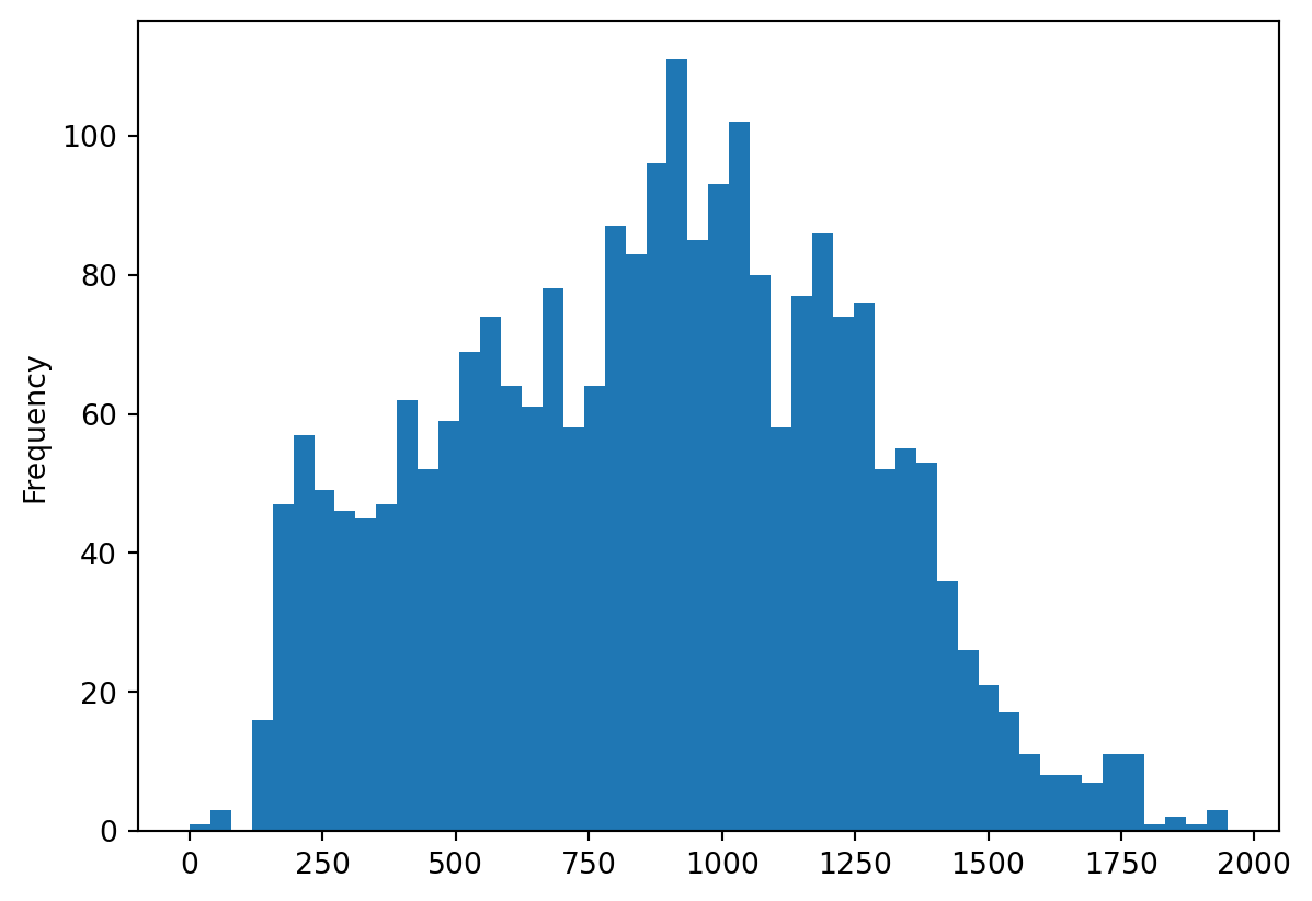
Maps in GeoPandas are of two kinds. Static images and interactive maps based on leaflet.js.
GeoPandas can also plot maps to check how the geometries appear in space. Call GeoDataFrame.plot() to plot the active geometry. To colour code by another column, pass in that column as the first argument. In the example below, you can plot the active geometry column and colour code by the "distance_to_arc" column. You may also want to show a legend (legend=True).
_ = buildings.plot("distance_to_arc", legend=True)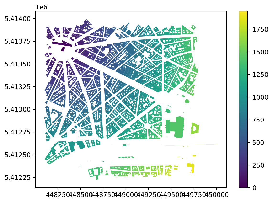
The map is created using the matplotlib package. It’s the same that was used under the hood for all the plots you have done before. You can use it directly to save the resulting plot to a PNG file.
1import matplotlib.pyplot as pltpyplot module of the matplotlib package as the plt alias.
If you now create the plot and use the plt.savefig() function in the same cell, a PNG will appear on your disk.
buildings.plot("distance_to_arc", legend=True)
plt.savefig("distance_to_arc.png", dpi=150)Some plots may not look as nice as the one above. The issue is that GeoPandas, by default, maps colors linearly between minimum and maximum. Check how would a plot showing building area look like.
_ = buildings.plot(buildings.area, legend=True)
This is not very useful. For this reason, GeoPandas allows you to pass a classification scheme to derive the bins for the colours from the distribution of values. For example, you can use quantiles.
_ = buildings.plot(buildings.area, scheme="quantiles", legend=True)
You can see some differentiation on a map now but it is not optimal. Other schemas might be better for this particular case, like Jenks-Caspall breaks. You can also specify the number of bins you want.
_ = buildings.plot(buildings.area, scheme="jenkscaspall", k=10, legend=True)
GeoPandas uses a package called mapclassify to do the classification schemes and you can check its documentation to see which are available (or create your own).
What happens when you apply a classification scheme is that GeoPandas derives bins from the distribution of your data using a selected algorithm. These are bins using the equal interval, which resembles the default linear mapping of colors.
import mapclassify
_ = mapclassify.classify(buildings.area, 'equal_interval').plot_legendgram(
inset=False, vlines=True, vlinecolor='red', cmap='viridis'
)
Quantiles would look like this.
_ = mapclassify.classify(buildings.area, 'quantiles').plot_legendgram(
inset=False, vlines=True, vlinecolor='red', cmap='viridis'
)
While Jenks Caspall breaks would do this:
_ = mapclassify.classify(buildings.area, 'jenkscaspall').plot_legendgram(
inset=False, vlines=True, vlinecolor='red', cmap='viridis'
)
The distribution you are dealing with has a very long tail, so the classification scheme needs to adapt.
Want to know more about static plots? Check this chapter of A Course on Geographic Data Science by Arribas-Bel (2019) or the GeoPandas documentation.
You can also explore your data interactively using GeoDataFrame.explore(), which behaves in the same way .plot() does but returns an interactive HTML map instead.
buildings.explore("distance_to_arc", legend=True)Using the GeoSeries of centroids, you can create a similar plot, but since you access only a single column, it has no values to show.
buildings["centroid"].explore()If you want to use centroids on a map but keep the data around to have them available in the tooltip, you can assign it as an active geometry and then use .explore().
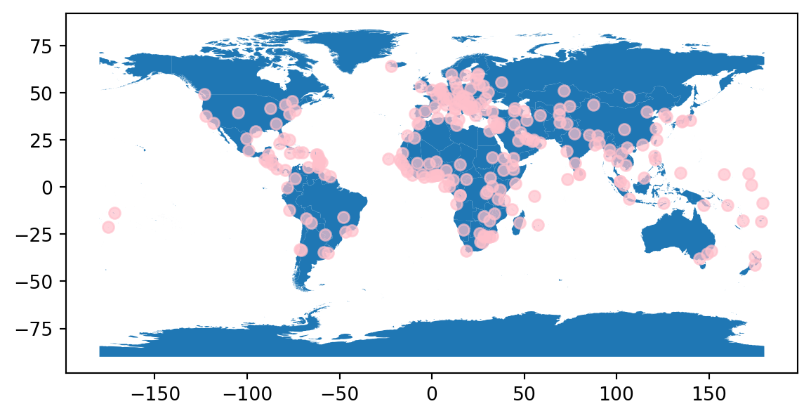
buildings.set_geometry("centroid").explore()You can also layer multiple geometry layers on top of each other. You just need to use one plot as a map (m) object for the others.
m) based on buildings. tiles="CartoDB Positron specifies which background tiles shall be used, popup=True enables pop-up (shows data on click) and tooltip=False disables tooltip (shows data on hover).
m=m ensures that both GeoDataFrames are shown on the same map.
color="pink" specifies the geometries’ colour if no data is shown.
marker_type="marker" specifies how points are shown on the map. Here, you want to use "marker".
m on the next line, the map will also be shown in the Notebook.
Now that you know how to plot, let’s get back to other constructive operation.
Geometry simplification is implemented using the simplify() and simplify_coverage() methods. The first one, simplifies each geometry on its own, while the latter one simplifies their shared boundaries together, preserving a valid coverage.
Using a pretty drastic simplification to illustrate the behavior, see how the individual simplification treats the data
simplified = buildings.simplify(10)
simplified.explore()The result no longer respects the original relations between individual buildings. This is different when using simplify_coverage(), which ensures that all the relations are retained.
simplified_coverage = buildings.simplify_coverage(10)
simplified_coverage.explore()Note that the method will work only when your data form a coverage and will struggle with overlapping polygons and similar situations.
Spatial predicates tell you the spatial relation between two geometries. Are they equal, intersect, overlap, or are they within another?
You have a location of Arc de Triomphe, allowing you to identify which of the buildings is the Arc. In other words, you can check which of the building polygons contain the Arc geometry.
1contains_arc = buildings.contains(arc.item())
contains_arc.head()item() returns the scalar object from a Series of length 1. Otherwise, GeoPandas would try to align two GeoSeries.
0 False
1 False
2 False
3 False
4 False
dtype: boolA predicate check like contains return a boolean array indicating the outcome of the check for each geometry. See if there is any True.
contains_arc.any()np.True_There is, so you can map it. The array can be passed directly to plot, no need to turn it into a column.
ax = buildings.plot(contains_arc, legend=True, cmap='coolwarm')
Get a point representing a location of another important building within the dataset - Grand Palais. As above, you can generate it directly from coordinates or using geocoding.
Directly:
palais = gpd.GeoSeries.from_xy(
x=[2.31222], y=[48.86616], crs="EPSG:4326"
).to_crs(buildings.crs)The code above uses known coordinates. If you don’t know them but know the address and a name of a place, you can use the built-in geocoding capabilities in geopandas:
palais = gpd.tools.geocode("Grand Palais, Paris").to_crs(buildings.crs)Then create a virtual straight line connecting the Arc de Triomphe and Grand Palais. Here comes one of those cases when you use shapely directly.
1palais_art = shapely.LineString([palais.geometry.item(), arc.geometry.item()])shapely.LineString geometry object with palais as a starting point and arc as an ending point.
Check visually what you have to get a better understanding.
ax = buildings.plot()
palais.plot(ax=ax, color='red')
arc.plot(ax=ax, color='orange')
gpd.GeoSeries([palais_art]).plot(ax=ax, color='k')
Now you can use another predicate check to figure out which buildings intersect this line.
intersects = buildings.intersects(palais_art)
buildings[intersects].plot()
Similarly, you can check all the budldings within a set distance from your line. Get those within 200 meters.
within_200 = buildings.dwithin(palais_art, 200)
buildings[within_200].plot()
The same could be done by buffering the line by 200 meters and doing the intersection check. However, using dwithin predicate directly is much more efficient.
Overlay operations can alter the data based on superimposition of two spatial layers.
The predicate checks above can filter all the buildings within a set distance. However, if you want to get only the areas strictly within the distance, you can clip the geometry.
1clipped_200 = buildings.clip(palais_art.buffer(200))
clipped_200.plot()clip method together with the buffered line.

The method takes all the geometries within the masking GeoSeries and returns only those portions of original that are contained within the mask.
Another overlay operation is spatial join. This does not alter geometry but attributes by joining attributes from one set of geometries to the other based on a spatial predicate (by default intersects).
Load the data capturing boundaries of Parisian Arrondissements (districts).
arrondissements = gpd.read_file(
'https://martinfleischmann.net/sds/geographic_data/data/arrondissements.geojson'
)
arrondissements.head(2)| n_sq_ar | c_ar | c_arinsee | l_ar | l_aroff | n_sq_co | surface | perimetre | geom_x_y | geometry | |
|---|---|---|---|---|---|---|---|---|---|---|
| 0 | 750000010 | 10 | 75110 | 10ème Ardt | Entrepôt | 750001537 | 2.891739e+06 | 6739.375055 | {'lon': 2.360728487847452, 'lat': 48.876130036... | POLYGON ((2.36469 48.88437, 2.36485 48.88436, ... |
| 1 | 750000018 | 18 | 75118 | 18ème Ardt | Buttes-Montmartre | 750001537 | 5.996051e+06 | 9916.464176 | {'lon': 2.3481605195620396, 'lat': 48.89256926... | POLYGON ((2.3658 48.88554, 2.36469 48.88437, 2... |
Instead of reading the file directly off the web, it is possible to download it manually, store it on your computer, and read it locally. To do that, you can follow these steps:
arrondissements = gpd.read_file(
"arrondissements.geojson",
)For any spatial overlay, you need to ensure that both layers share the CRS.
arrondissements.crs.equals(buildings.crs)FalseGiven that is not the case, re-project.
arrondissements = arrondissements.to_crs(buildings.crs)Now you can check how these two GeoDataFrames relate to each other.
ax = buildings.plot()
arrondissements.boundary.plot(ax=ax, color='red')
Buildings are on the boundary of four arrondissements. Use spatial join to link the information about the arrondissement to each building geometry.
buildings_joined = buildings.sjoin(arrondissements)
buildings_joined.head()| uID | blg_area | wall | adjacency | neighbour_distance | nID | length | linearity | width | width_deviation | ... | index_right | n_sq_ar | c_ar | c_arinsee | l_ar | l_aroff | n_sq_co | surface | perimetre | geom_x_y | |
|---|---|---|---|---|---|---|---|---|---|---|---|---|---|---|---|---|---|---|---|---|---|
| 0 | 0 | 27194.254623 | 1079.492255 | 0.423913 | 79.492252 | 1 | 238.865434 | 0.999987 | 50.00000 | 0.000000 | ... | 14 | 750000008 | 8 | 75108 | 8ème Ardt | Élysée | 750001537 | 3.880036e+06 | 7880.533268 | {'lon': 2.312554022402065, 'lat': 48.872720837... |
| 1 | 1 | 2196.125585 | 255.198183 | 0.857143 | 52.080293 | 17 | 213.373518 | 0.999935 | 40.47981 | 0.580373 | ... | 10 | 750000007 | 7 | 75107 | 7ème Ardt | Palais-Bourbon | 750001537 | 4.090057e+06 | 8099.424883 | {'lon': 2.3121876953655494, 'lat': 48.85617443... |
| 2 | 2 | 34.882075 | 39.461749 | 0.583333 | 49.413639 | 17 | 213.373518 | 0.999935 | 40.47981 | 0.580373 | ... | 10 | 750000007 | 7 | 75107 | 7ème Ardt | Palais-Bourbon | 750001537 | 4.090057e+06 | 8099.424883 | {'lon': 2.3121876953655494, 'lat': 48.85617443... |
| 3 | 3 | 38.808817 | 39.461749 | 0.600000 | 43.450128 | 17 | 213.373518 | 0.999935 | 40.47981 | 0.580373 | ... | 10 | 750000007 | 7 | 75107 | 7ème Ardt | Palais-Bourbon | 750001537 | 4.090057e+06 | 8099.424883 | {'lon': 2.3121876953655494, 'lat': 48.85617443... |
| 4 | 4 | 90.426163 | 255.198183 | 0.833333 | 12.131337 | 17 | 213.373518 | 0.999935 | 40.47981 | 0.580373 | ... | 10 | 750000007 | 7 | 75107 | 7ème Ardt | Palais-Bourbon | 750001537 | 4.090057e+06 | 8099.424883 | {'lon': 2.3121876953655494, 'lat': 48.85617443... |
5 rows × 31 columns
All of the columns from the arrondissements GeoDataFrame are now linked to the buildings GeoDataFrame with values derived based on the intersection of geometries. This allows you to plot the arrondissement information on building geometry.
buildings_joined.plot('l_ar', legend=True)
A use case that may come after a join like this is to combine all individual geometries from each arrondissement to single one, dissolving the boundaries where they touch. An operation like this can be done using the dissolve method.
1arr_buildings_combined = buildings_joined.dissolve('l_ar')
arr_buildings_combined| geometry | uID | blg_area | wall | adjacency | neighbour_distance | nID | length | linearity | width | ... | distance_to_arc | index_right | n_sq_ar | c_ar | c_arinsee | l_aroff | n_sq_co | surface | perimetre | geom_x_y | |
|---|---|---|---|---|---|---|---|---|---|---|---|---|---|---|---|---|---|---|---|---|---|
| l_ar | |||||||||||||||||||||
| 16ème Ardt | MULTIPOLYGON (((448146.481 5412398.673, 448139... | 1390 | 425.107877 | 195.330383 | 0.408163 | 14.919710 | 255 | 117.129504 | 0.983358 | 37.070298 | ... | 1081.057878 | 4 | 750000016 | 16 | 75116 | Passy | 750001537 | 1.637254e+07 | 17416.109657 | {'lon': 2.261970788364543, 'lat': 48.860392105... |
| 17ème Ardt | MULTIPOLYGON (((448204.628 5413753.609, 448194... | 1387 | 18.136715 | 18.302225 | 0.523810 | 25.766580 | 106 | 99.567245 | 0.999982 | 24.040316 | ... | 130.771660 | 7 | 750000017 | 17 | 75117 | Batignolles-Monceau | 750001537 | 5.668835e+06 | 10775.579516 | {'lon': 2.3067769905744084, 'lat': 48.88732652... |
| 7ème Ardt | MULTIPOLYGON (((448878.802 5412279.488, 448878... | 1 | 2196.125585 | 255.198183 | 0.857143 | 52.080293 | 17 | 213.373518 | 0.999935 | 40.479810 | ... | 1905.389066 | 10 | 750000007 | 7 | 75107 | Palais-Bourbon | 750001537 | 4.090057e+06 | 8099.424883 | {'lon': 2.3121876953655494, 'lat': 48.85617443... |
| 8ème Ardt | MULTIPOLYGON (((448574.149 5413168.587, 448566... | 0 | 27194.254623 | 1079.492255 | 0.423913 | 79.492252 | 1 | 238.865434 | 0.999987 | 50.000000 | ... | 1422.562389 | 14 | 750000008 | 8 | 75108 | Élysée | 750001537 | 3.880036e+06 | 7880.533268 | {'lon': 2.312554022402065, 'lat': 48.872720837... |
4 rows × 30 columns
As you can see, the buildings are now combined to a single MultiPolygon per each arrondissement. This may not be optimal, so you can explode them to individual Polygons.
arr_buildings = arr_buildings_combined.explode()
arr_buildings.head(2)| uID | blg_area | wall | adjacency | neighbour_distance | nID | length | linearity | width | width_deviation | ... | index_right | n_sq_ar | c_ar | c_arinsee | l_aroff | n_sq_co | surface | perimetre | geom_x_y | geometry | |
|---|---|---|---|---|---|---|---|---|---|---|---|---|---|---|---|---|---|---|---|---|---|
| l_ar | |||||||||||||||||||||
| 16ème Ardt | 1390 | 425.107877 | 195.330383 | 0.408163 | 14.91971 | 255 | 117.129504 | 0.983358 | 37.070298 | 3.326807 | ... | 4 | 750000016 | 16 | 75116 | Passy | 750001537 | 1.637254e+07 | 17416.109657 | {'lon': 2.261970788364543, 'lat': 48.860392105... | POLYGON ((448146.481 5412398.673, 448139.954 5... |
| 16ème Ardt | 1390 | 425.107877 | 195.330383 | 0.408163 | 14.91971 | 255 | 117.129504 | 0.983358 | 37.070298 | 3.326807 | ... | 4 | 750000016 | 16 | 75116 | Passy | 750001537 | 1.637254e+07 | 17416.109657 | {'lon': 2.261970788364543, 'lat': 48.860392105... | POLYGON ((448153.588 5412419.874, 448155.901 5... |
2 rows × 30 columns
The resulting geometry reflects a dissolution (merge) of all buildings that are connected. This could’ve been done directly as well but that would not allow us to illustrate dissolve by a column.
arr_buildings.explore()