Data wrangling

You know the basics. What are Jupyter notebooks, how do they work, and how do you run Python in them. It is time to start using them for data science (no, that simple math you did the last time doesn’t count as data science).

You are about to enter the PyData ecosystem. It means that you will start learning how to work with Python from the middle. This course does not explicitly cover the fundamentals of programming. It is expected that those parts you need you’ll be able to pick as you go through the specialised data science stack. If you’re stuck, confused or need further explanation, use Google (or your favourite search engine), ask AI to explain the code or ask in online chat or during the class. Not everything will be told during the course (by design), and the internet is a friend of every programmer, so let’s figure out how to use it efficiently from the beginning.

Let’s dig in!

Munging and wrangling

Real-world datasets are messy. There is no way around it: datasets have “holes” (missing data), the amount of formats in which data can be stored is endless, and the best structure to share data is not always the optimum to analyse them, hence the need to munge ¹ them. As has been correctly pointed out in many outlets, much of the time spent in what is called Data Science is related not only to sophisticated modelling and insight but has to do with much more basic and less exotic tasks such as obtaining data, processing, and turning them into a shape that makes analysis possible, and exploring it to get to know their basic properties.

Surprisingly, very little has been published on patterns, techniques, and best practices for quick and efficient data cleaning, manipulation, and transformation because of how labour-intensive and relevant this aspect is. In this session, you will use a few real-world datasets and learn how to process them into Python so they can be transformed and manipulated, if necessary, and analysed. For this, you will introduce some of the bread and butter of data analysis and scientific computing in Python. These are fundamental tools that are constantly used in almost any task relating to data analysis.

This notebook covers the basics and the content that is expected to be learnt by every student. You use a prepared dataset that saves us much of the more intricate processing that goes beyond the introductory level the session is aimed at. If you are interested in how it was done, there is a notebook.

This notebook discusses several patterns to clean and structure data properly, including tidying, subsetting, and aggregating. You finish with some basic visualisation. An additional extension presents more advanced tricks to manipulate tabular data.

Dataset

You will be exploring demographic characteristics of Chicago in 1918 linked to the influenza mortality during the pandemic that happened back then, coming from the research paper by Grantz et al. (2016). The data are aggregated to census tracts and contain information on unemployment, home ownership, age structure and influenza mortality from a period of 8 weeks.

The main tool you use is the pandas package. As with the math you used before, you must import it first.

1import pandas as pd

1: Import the pandas package under the alias pd. Using the alias is not necessary, but it is a convention nearly everyone follows.

The data is stored in a CSV file. To make things easier, you can read data from a file posted online so, for now, you do not need to download any dataset:

1chicago_1918 = pd.read_csv(
2    "https://martinfleischmann.net/sds/data_wrangling/data/chicago_influenza_1918.csv",
3    index_col="geography_code",
)

1: Use the read_csv function from pandas. Remember that you have imported pandas as pd.
2: Specify the path to the file. It could be a web address like here or a local file path.
3: Use the column geography_code as an index of the table by passing its name to the index_col keyword argument. It is not strictly necessary but allows us to choose and index on reading instead of specifying it later. More on indices below.

Tip

You are using read_csv because the file you want to read is in CSV format. However, pandas allows for many more formats to be read and write. A full list of formats supported may be found in the documentation.

Alternative

Instead of reading the file directly off the web, it is possible to download it manually, store it on your computer, and read it locally. To do that, you can follow these steps:

Download the file by right-clicking on this link and saving the file
Place the file in the same folder as the notebook where you intend to read it
Replace the code in the cell above with:

chicago_1918 = pd.read_csv(
    "chicago_influenza_1918.csv",
    index_col="geography_code",
)

Pandas 101

Now, you are ready to start playing and interrogating the dataset! What you have at your fingertips is a table summarising, for each of the census tracts in Chicago more than a century ago, how many people lived in each by age, accompanied by some other socioeconomic data and influenza mortality. These tables are called DataFrame objects, and they have a lot of functionality built-in to explore and manipulate the data they contain. Let’s explore a few of those cool tricks!

Data Structures

The first aspect worth spending a bit of time on is the structure of a DataFrame. You can print it by simply typing its name:

chicago_1918

	gross_acres	illit	unemployed_pct	ho_pct	agecat1	agecat2	agecat3	agecat4	agecat5	agecat6	agecat7	influenza
geography_code
G17003100001	1388.2	116	0.376950	0.124823	46	274	257	311	222	1122	587	9
G17003100002	217.7	14	0.399571	0.071647	35	320	441	624	276	1061	508	6
G17003100003	401.3	69	0.349558	0.092920	50	265	179	187	163	1020	392	8
G17003100004	86.9	11	0.422535	0.030072	43	241	129	141	123	1407	539	2
G17003100005	337.1	20	0.431822	0.084703	65	464	369	464	328	2625	1213	7
...	...	...	...	...	...	...	...	...	...	...	...	...
G17003100492	2176.6	136	0.404430	0.173351	85	606	520	705	439	2141	1460	12
G17003100493	680.0	271	0.377207	0.130158	243	1349	957	1264	957	4653	2180	40
G17003100494	1392.8	1504	0.336032	0.072317	309	1779	1252	1598	1086	6235	2673	85
G17003100495	640.0	167	0.311917	0.085667	59	333	206	193	80	726	224	15
G17003100496	709.8	340	0.369765	0.113549	157	979	761	959	594	2862	1206	30

496 rows × 12 columns

Note the printing is cut to keep a nice and compact view but enough to see its structure. Since they represent a table of data, DataFrame objects have two dimensions: rows and columns. Each of these is automatically assigned a name in what you will call its index. When printing, the index of each dimension is rendered in bold, as opposed to the standard rendering for the content. The example above shows how the column index is automatically picked up from the .csv file’s column names. For rows, we have specified when reading the file you wanted the column geography_code, so that is used. If you hadn’t set any, pandas would automatically generate a sequence starting in 0 and going all the way to the number of rows minus one. This is the standard structure of a DataFrame object, so you will come to it over and over. Importantly, even when you move to spatial data, your datasets will have a similar structure.

One final feature that is worth mentioning about these tables is that they can hold columns with different types of data. In this example, you have counts (or int for integer types) and ratios (or ‘float’ for floating point numbers - a number with decimals) for each column. But it is useful to keep in mind that you can combine this with columns that hold other types of data such as categories, text (str, for string), dates or, as you will see later in the course, geographic features.

To extract a single column from this DataFrame, specify its name in the square brackets ([]). Note that the name, in this case, is a string. A piece of text. As such, it needs to be within single (') or double quotes ("). The resulting data structure is no longer a DataFrame, but you have a Series because you deal with a single column.

chicago_1918["influenza"]

geography_code
G17003100001     9
G17003100002     6
G17003100003     8
G17003100004     2
G17003100005     7
                ..
G17003100492    12
G17003100493    40
G17003100494    85
G17003100495    15
G17003100496    30
Name: influenza, Length: 496, dtype: int64

Inspect

Inspecting what it looks like. You can check the table’s top (or bottom) X lines by passing X to the method head (tail). For example, for the top/bottom five lines:

chicago_1918.head()

	gross_acres	illit	unemployed_pct	ho_pct	agecat1	agecat2	agecat3	agecat4	agecat5	agecat6	agecat7	influenza
geography_code
G17003100001	1388.2	116	0.376950	0.124823	46	274	257	311	222	1122	587	9
G17003100002	217.7	14	0.399571	0.071647	35	320	441	624	276	1061	508	6
G17003100003	401.3	69	0.349558	0.092920	50	265	179	187	163	1020	392	8
G17003100004	86.9	11	0.422535	0.030072	43	241	129	141	123	1407	539	2
G17003100005	337.1	20	0.431822	0.084703	65	464	369	464	328	2625	1213	7

chicago_1918.tail()

	gross_acres	illit	unemployed_pct	ho_pct	agecat1	agecat2	agecat3	agecat4	agecat5	agecat6	agecat7	influenza
geography_code
G17003100492	2176.6	136	0.404430	0.173351	85	606	520	705	439	2141	1460	12
G17003100493	680.0	271	0.377207	0.130158	243	1349	957	1264	957	4653	2180	40
G17003100494	1392.8	1504	0.336032	0.072317	309	1779	1252	1598	1086	6235	2673	85
G17003100495	640.0	167	0.311917	0.085667	59	333	206	193	80	726	224	15
G17003100496	709.8	340	0.369765	0.113549	157	979	761	959	594	2862	1206	30

Or get an overview of the table:

chicago_1918.info()

<class 'pandas.core.frame.DataFrame'>
Index: 496 entries, G17003100001 to G17003100496
Data columns (total 12 columns):
 #   Column          Non-Null Count  Dtype  
---  ------          --------------  -----  
 0   gross_acres     496 non-null    float64
 1   illit           496 non-null    int64  
 2   unemployed_pct  496 non-null    float64
 3   ho_pct          496 non-null    float64
 4   agecat1         496 non-null    int64  
 5   agecat2         496 non-null    int64  
 6   agecat3         496 non-null    int64  
 7   agecat4         496 non-null    int64  
 8   agecat5         496 non-null    int64  
 9   agecat6         496 non-null    int64  
 10  agecat7         496 non-null    int64  
 11  influenza       496 non-null    int64  
dtypes: float64(3), int64(9)
memory usage: 66.5+ KB

Summarise

Or of the values of the table:

chicago_1918.describe()

	gross_acres	illit	unemployed_pct	ho_pct	agecat1	agecat2	agecat3	agecat4	agecat5	agecat6	agecat7	influenza
count	496.000000	496.000000	496.000000	496.000000	496.000000	496.000000	496.000000	496.000000	496.000000	496.000000	496.000000	496.000000
mean	233.245968	199.116935	0.345818	0.061174	102.370968	555.167339	406.560484	524.100806	416.044355	2361.582661	1052.681452	16.070565
std	391.630857	297.836201	0.050498	0.038189	78.677423	423.526444	301.564896	369.875444	281.825682	1545.469426	722.955717	12.252440
min	6.900000	0.000000	0.057800	0.000000	0.000000	3.000000	1.000000	4.000000	0.000000	8.000000	6.000000	0.000000
25%	79.975000	30.750000	0.323973	0.032106	46.750000	256.500000	193.500000	253.750000	220.500000	1169.750000	519.750000	8.000000
50%	99.500000	84.000000	0.353344	0.054389	82.000000	442.500000	331.500000	453.500000	377.000000	2102.000000	918.500000	13.500000
75%	180.125000	241.250000	0.373382	0.084762	136.000000	717.500000	532.500000	709.500000	551.750000	3191.750000	1379.250000	21.000000
max	3840.000000	2596.000000	0.495413	0.197391	427.000000	2512.000000	1917.000000	2665.000000	2454.000000	9792.000000	4163.000000	85.000000

Note how the output is also a DataFrame object, so you can do with it the same things you would with the original table (e.g. writing it to a file).

In this case, the summary might be better presented if the table is “transposed”:

chicago_1918.describe().T

	count	mean	std	min	25%	50%	75%	max
gross_acres	496.0	233.245968	391.630857	6.9000	79.975000	99.500000	180.125000	3840.000000
illit	496.0	199.116935	297.836201	0.0000	30.750000	84.000000	241.250000	2596.000000
unemployed_pct	496.0	0.345818	0.050498	0.0578	0.323973	0.353344	0.373382	0.495413
ho_pct	496.0	0.061174	0.038189	0.0000	0.032106	0.054389	0.084762	0.197391
agecat1	496.0	102.370968	78.677423	0.0000	46.750000	82.000000	136.000000	427.000000
agecat2	496.0	555.167339	423.526444	3.0000	256.500000	442.500000	717.500000	2512.000000
agecat3	496.0	406.560484	301.564896	1.0000	193.500000	331.500000	532.500000	1917.000000
agecat4	496.0	524.100806	369.875444	4.0000	253.750000	453.500000	709.500000	2665.000000
agecat5	496.0	416.044355	281.825682	0.0000	220.500000	377.000000	551.750000	2454.000000
agecat6	496.0	2361.582661	1545.469426	8.0000	1169.750000	2102.000000	3191.750000	9792.000000
agecat7	496.0	1052.681452	722.955717	6.0000	519.750000	918.500000	1379.250000	4163.000000
influenza	496.0	16.070565	12.252440	0.0000	8.000000	13.500000	21.000000	85.000000

Equally, common descriptive statistics are also available. To obtain minimum values for each column, you can use .min().

chicago_1918.min()

gross_acres       6.9000
illit             0.0000
unemployed_pct    0.0578
ho_pct            0.0000
agecat1           0.0000
agecat2           3.0000
agecat3           1.0000
agecat4           4.0000
agecat5           0.0000
agecat6           8.0000
agecat7           6.0000
influenza         0.0000
dtype: float64

Or to obtain a minimum for a single column only.

chicago_1918["influenza"].min()

Note here how you have restricted the calculation of the minimum value to one column only by getting the Series and calling .min() on that.

Similarly, you can restrict the calculations to a single row using .loc[] indexer:

chicago_1918.loc["G17003100492"].max()

2176.6

Create new columns

You can generate new variables by applying operations to existing ones. For example, you can calculate the total population by area. Here are a couple of ways to do it:

# This one is longer, hardcoded
1total_population = (
2    chicago_1918["agecat1"]
    + chicago_1918["agecat2"]
    + chicago_1918["agecat3"]
    + chicago_1918["agecat4"]
    + chicago_1918["agecat5"]
    + chicago_1918["agecat6"]
    + chicago_1918["agecat7"]
)
3total_population.head()

1: Create a new variable called total_population to store the result.
2: Select all the columns and add them together
3: Print the top of the variable

geography_code
G17003100001    2819
G17003100002    3265
G17003100003    2256
G17003100004    2623
G17003100005    5528
dtype: int64

# This one is shorted, using a range of columns and sum
1total_population = chicago_1918.loc[:, "agecat1":"agecat7"].sum(axis=1)
total_population.head()

1: This line is simple, but a lot happens here. Using .loc[], you select all the rows (: part) and all the columns between "agecat1" and "agecat7". Then you apply .sum() over axis=1, which means along rows, to get a sum per each row.

geography_code
G17003100001    2819
G17003100002    3265
G17003100003    2256
G17003100004    2623
G17003100005    5528
dtype: int64

Once you have created the variable, you can make it part of the table:

1chicago_1918["total_population"] = total_population
chicago_1918.head()

1: Assing a variable total_population that contains a Series as a column "total_population". pandas creates that column automatically. If it existed, it would get overridden.

	gross_acres	illit	unemployed_pct	ho_pct	agecat1	agecat2	agecat3	agecat4	agecat5	agecat6	agecat7	influenza	total_population
geography_code
G17003100001	1388.2	116	0.376950	0.124823	46	274	257	311	222	1122	587	9	2819
G17003100002	217.7	14	0.399571	0.071647	35	320	441	624	276	1061	508	6	3265
G17003100003	401.3	69	0.349558	0.092920	50	265	179	187	163	1020	392	8	2256
G17003100004	86.9	11	0.422535	0.030072	43	241	129	141	123	1407	539	2	2623
G17003100005	337.1	20	0.431822	0.084703	65	464	369	464	328	2625	1213	7	5528

You can also do other mathematical operations on columns. These are always automatically applied to individual values in corresponding rows.

1homeowners = chicago_1918["total_population"] * chicago_1918["ho_pct"]
homeowners.head()

1: A product of the total population and home ownership percentage provides an estimation of the number of homeowners per census tract.

geography_code
G17003100001    351.875177
G17003100002    233.928353
G17003100003    209.628319
G17003100004     78.879711
G17003100005    468.237675
dtype: float64

1pop_density = chicago_1918["total_population"] / chicago_1918["gross_acres"]
pop_density.head()

1: A division of the total population by the area results in an estimation of the population density.

geography_code
G17003100001     2.030687
G17003100002    14.997703
G17003100003     5.621729
G17003100004    30.184120
G17003100005    16.398695
dtype: float64

A different spin on this is assigning new values: you can generate new variables with scalars², and modify those:

1chicago_1918["ones"] = 1
chicago_1918.head()

1: Create a new column named "ones" with all ones.

	gross_acres	illit	unemployed_pct	ho_pct	agecat1	agecat2	agecat3	agecat4	agecat5	agecat6	agecat7	influenza	total_population	ones
geography_code
G17003100001	1388.2	116	0.376950	0.124823	46	274	257	311	222	1122	587	9	2819	1
G17003100002	217.7	14	0.399571	0.071647	35	320	441	624	276	1061	508	6	3265	1
G17003100003	401.3	69	0.349558	0.092920	50	265	179	187	163	1020	392	8	2256	1
G17003100004	86.9	11	0.422535	0.030072	43	241	129	141	123	1407	539	2	2623	1
G17003100005	337.1	20	0.431822	0.084703	65	464	369	464	328	2625	1213	7	5528	1

And you can modify specific values too:

chicago_1918.loc["G17003100001", "ones"] = 3
chicago_1918.head()

	gross_acres	illit	unemployed_pct	ho_pct	agecat1	agecat2	agecat3	agecat4	agecat5	agecat6	agecat7	influenza	total_population	ones
geography_code
G17003100001	1388.2	116	0.376950	0.124823	46	274	257	311	222	1122	587	9	2819	3
G17003100002	217.7	14	0.399571	0.071647	35	320	441	624	276	1061	508	6	3265	1
G17003100003	401.3	69	0.349558	0.092920	50	265	179	187	163	1020	392	8	2256	1
G17003100004	86.9	11	0.422535	0.030072	43	241	129	141	123	1407	539	2	2623	1
G17003100005	337.1	20	0.431822	0.084703	65	464	369	464	328	2625	1213	7	5528	1

Remove columns

Permanently deleting variables is also within reach of one command:

chicago_1918 = chicago_1918.drop(columns="ones")
chicago_1918.head()

	gross_acres	illit	unemployed_pct	ho_pct	agecat1	agecat2	agecat3	agecat4	agecat5	agecat6	agecat7	influenza	total_population
geography_code
G17003100001	1388.2	116	0.376950	0.124823	46	274	257	311	222	1122	587	9	2819
G17003100002	217.7	14	0.399571	0.071647	35	320	441	624	276	1061	508	6	3265
G17003100003	401.3	69	0.349558	0.092920	50	265	179	187	163	1020	392	8	2256
G17003100004	86.9	11	0.422535	0.030072	43	241	129	141	123	1407	539	2	2623
G17003100005	337.1	20	0.431822	0.084703	65	464	369	464	328	2625	1213	7	5528

Index-based queries

Here, you explore how to subset parts of a DataFrame if you know exactly which bits you want. For example, if you want to extract the influenza mortality and total population of the first four areas in the table, you use loc with lists:

1death_pop_first4 = chicago_1918.loc[
2    ["G17003100001", "G17003100002", "G17003100003", "G17003100004"],
3    ["influenza", "total_population"],
]
death_pop_first4

1: loc takes two inputs. Selection of rows and selection of columns. If the latter is not present, it is assumed that all the columns are selected. The same could be achieved by using :.
2: A list of index values. Note that you use squared brackets ([]) to delineate the index of the items you want to subset. In Python, this sequence of items is called a list.
3: A list of columns.

	influenza	total_population
geography_code
G17003100001	9	2819
G17003100002	6	3265
G17003100003	8	2256
G17003100004	2	2623

You can see how you can create a list with the names (index IDs) along each of the two dimensions of a DataFrame (rows and columns), and loc will return a subset of the original table only with the elements queried for.

An alternative to list-based queries is what is called “range-based” queries. These work on the indices of the table, but instead of requiring the ID of each item you want to retrieve, they operate by requiring only two IDs: the first and last element in a range of items. Range queries are expressed with a colon (:). For example:

range_query = chicago_1918.loc[
    "G17003100010":"G17003100012",
    "influenza":'total_population',
]
range_query

	influenza	total_population
geography_code
G17003100010	18	11380
G17003100011	16	8382
G17003100012	8	5874

The range query picks up all the elements between the specified IDs. Note that for this to work, the first ID in the range needs to be placed before the second one in the table’s index.

Once you know about list and range-based queries, you can combine them! For example, you can specify a range of rows and a list of columns:

range_list_qry = chicago_1918.loc[
    "G17003100010":"G17003100012", ["influenza", "total_population"]
]

range_list_qry

	influenza	total_population
geography_code
G17003100010	18	11380
G17003100011	16	8382
G17003100012	8	5874

Condition-based queries

However, sometimes, you do not know exactly which observations you want, but you do know what conditions they need to satisfy (e.g. areas with more than 2,000 inhabitants). For these cases, DataFrames support selection based on conditions. Let us see a few examples. Suppose you want to select…

… areas with more than 60 cases of influenza deaths:

flu_over_60 = chicago_1918.loc[chicago_1918["influenza"] > 60]
flu_over_60

	gross_acres	illit	unemployed_pct	ho_pct	agecat1	agecat2	agecat3	agecat4	agecat5	agecat6	agecat7	influenza	total_population
geography_code
G17003100196	80.5	951	0.301564	0.016648	228	1504	925	998	608	3583	1092	62	8938
G17003100246	113.0	2596	0.330517	0.027537	407	2090	1497	1681	1063	4564	1934	77	13236
G17003100247	91.1	1534	0.293748	0.020664	215	1136	770	775	530	2993	1152	61	7571
G17003100285	120.0	621	0.318677	0.047779	419	1870	1190	1263	818	4370	1335	82	11265
G17003100352	600.0	638	0.267962	0.055023	404	1962	1251	1151	603	5261	1251	70	11883
G17003100494	1392.8	1504	0.336032	0.072317	309	1779	1252	1598	1086	6235	2673	85	14932

… areas with less than 200 inhabitants:

pop_under = chicago_1918.loc[chicago_1918["total_population"] < 200]
pop_under

	gross_acres	illit	unemployed_pct	ho_pct	agecat1	agecat2	agecat3	agecat4	agecat5	agecat6	agecat7	influenza	total_population
geography_code
G17003100093	71.2	34	0.268041	0.025773	4	33	20	25	10	66	36	0	194
G17003100293	40.0	17	0.345238	0.053571	4	23	18	26	16	59	22	0	168
G17003100297	38.1	4	0.461538	0.000000	0	3	1	4	0	8	10	0	26
G17003100353	320.0	28	0.193750	0.018750	1	7	4	10	12	80	46	2	160
G17003100488	1600.1	3	0.404762	0.000000	2	5	4	7	1	17	6	0	42

… areas with exactly a hundred illiterate persons:

illit_100 = chicago_1918.loc[chicago_1918["illit"] == 100]
illit_100

	gross_acres	illit	unemployed_pct	ho_pct	agecat1	agecat2	agecat3	agecat4	agecat5	agecat6	agecat7	influenza	total_population
geography_code
G17003100076	79.4	100	0.326936	0.043691	140	791	562	666	520	3163	1496	20	7338
G17003100483	670.0	100	0.379153	0.142368	188	1170	829	1132	763	3191	1482	21	8755

Unlimited power

These queries can grow in sophistication with almost no limits. For example, here is a case where you want to find out the areas where the oldest age group is more than half the population:

chicago_1918.loc[
    (chicago_1918["agecat7"] * 100 / chicago_1918["total_population"]) > 50
]

	gross_acres	illit	unemployed_pct	ho_pct	agecat1	agecat2	agecat3	agecat4	agecat5	agecat6	agecat7	influenza	total_population
geography_code
G17003100227	146.3	22	0.0657	0.000853	2	16	9	22	27	480	614	3	1170

All the condition-based queries above are expressed using the loc operator. This is a powerful way, and since it shares syntax with index-based queries, it is also easier to remember. However, sometimes querying using loc involves a lot of quotation marks, parenthesis, etc. A more streamlined approach for condition-based queries of rows is provided by the query engine. Using this approach, you express everything in our query on a single string, or piece of text, and that is evaluated in the table at once. For example, you can run the same operation as in the first query above with the following syntax:

flu_over_60_query = chicago_1918.query("influenza > 60")
flu_over_60_query

	gross_acres	illit	unemployed_pct	ho_pct	agecat1	agecat2	agecat3	agecat4	agecat5	agecat6	agecat7	influenza	total_population
geography_code
G17003100196	80.5	951	0.301564	0.016648	228	1504	925	998	608	3583	1092	62	8938
G17003100246	113.0	2596	0.330517	0.027537	407	2090	1497	1681	1063	4564	1934	77	13236
G17003100247	91.1	1534	0.293748	0.020664	215	1136	770	775	530	2993	1152	61	7571
G17003100285	120.0	621	0.318677	0.047779	419	1870	1190	1263	818	4370	1335	82	11265
G17003100352	600.0	638	0.267962	0.055023	404	1962	1251	1151	603	5261	1251	70	11883
G17003100494	1392.8	1504	0.336032	0.072317	309	1779	1252	1598	1086	6235	2673	85	14932

If you want to combine operations, this is also possible:

flu_query = chicago_1918.query("(influenza > 60) & (total_population < 10000)")
flu_query

	gross_acres	illit	unemployed_pct	ho_pct	agecat1	agecat2	agecat3	agecat4	agecat5	agecat6	agecat7	influenza	total_population
geography_code
G17003100196	80.5	951	0.301564	0.016648	228	1504	925	998	608	3583	1092	62	8938
G17003100247	91.1	1534	0.293748	0.020664	215	1136	770	775	530	2993	1152	61	7571

Note that, in these cases, using query results in code that is much more streamlined and easier to read. However, query is not perfect and, particularly for more sophisticated queries, it does not afford the same degree of flexibility. For example, the last query we had using loc would not be possible using query.

Tip

If you are interested, more detail about query is available in the pandas documentation.

Combining queries

Now, all of these queries can be combined with each other for further flexibility. For example, imagine you want areas with more than 60 cases of influenza from areas with less than 10,000 inhabitants:

flu_loc = chicago_1918.loc[
    (chicago_1918["influenza"] > 60)
1    & (chicago_1918["total_population"] < 10000)
]
flu_loc

1: The & operator combines both conditions together.

	gross_acres	illit	unemployed_pct	ho_pct	agecat1	agecat2	agecat3	agecat4	agecat5	agecat6	agecat7	influenza	total_population
geography_code
G17003100196	80.5	951	0.301564	0.016648	228	1504	925	998	608	3583	1092	62	8938
G17003100247	91.1	1534	0.293748	0.020664	215	1136	770	775	530	2993	1152	61	7571

How do the loc queries work?

Let’s unpack how these queries work. Each part of the query above creates a single Series with boolean (True or False) values, encoding whether the row fulfils the condition or not.

chicago_1918["influenza"] > 60

geography_code
G17003100001    False
G17003100002    False
G17003100003    False
G17003100004    False
G17003100005    False
                ...  
G17003100492    False
G17003100493    False
G17003100494     True
G17003100495    False
G17003100496    False
Name: influenza, Length: 496, dtype: bool

chicago_1918["total_population"] < 10000

geography_code
G17003100001     True
G17003100002     True
G17003100003     True
G17003100004     True
G17003100005     True
                ...  
G17003100492     True
G17003100493    False
G17003100494    False
G17003100495     True
G17003100496     True
Name: total_population, Length: 496, dtype: bool

You then combine two of these Series with &, asking for a new Series where values in both the first and the second Series are True.

(chicago_1918["influenza"] > 60) & (chicago_1918["total_population"] < 10000)

geography_code
G17003100001    False
G17003100002    False
G17003100003    False
G17003100004    False
G17003100005    False
                ...  
G17003100492    False
G17003100493    False
G17003100494    False
G17003100495    False
G17003100496    False
Length: 496, dtype: bool

Such a Series is then essentially used as a mask, and loc returns only those columns that contain True in that mask.

Sorting

Among the many operations DataFrame objects support, one of the most useful ones is to sort a table based on a given column. For example, imagine you want to sort the table by the influenza cases:

1chicago_sorted = chicago_1918.sort_values('influenza', ascending=False)
chicago_sorted

1: By default, pandas is sorting from the smallest to the largest values (ascending). By specifying ascending=False, you switch the order.

	gross_acres	illit	unemployed_pct	ho_pct	agecat1	agecat2	agecat3	agecat4	agecat5	agecat6	agecat7	influenza	total_population
geography_code
G17003100494	1392.8	1504	0.336032	0.072317	309	1779	1252	1598	1086	6235	2673	85	14932
G17003100285	120.0	621	0.318677	0.047779	419	1870	1190	1263	818	4370	1335	82	11265
G17003100246	113.0	2596	0.330517	0.027537	407	2090	1497	1681	1063	4564	1934	77	13236
G17003100352	600.0	638	0.267962	0.055023	404	1962	1251	1151	603	5261	1251	70	11883
G17003100196	80.5	951	0.301564	0.016648	228	1504	925	998	608	3583	1092	62	8938
...	...	...	...	...	...	...	...	...	...	...	...	...	...
G17003100396	26.2	8	0.344066	0.015639	14	54	31	53	48	609	275	0	1084
G17003100293	40.0	17	0.345238	0.053571	4	23	18	26	16	59	22	0	168
G17003100488	1600.1	3	0.404762	0.000000	2	5	4	7	1	17	6	0	42
G17003100297	38.1	4	0.461538	0.000000	0	3	1	4	0	8	10	0	26
G17003100093	71.2	34	0.268041	0.025773	4	33	20	25	10	66	36	0	194

496 rows × 13 columns

Given the areas of each census tract differ, it may be better to sort by the mortality rate rather than raw counts.

1chicago_1918["flu_rate"] = (
    chicago_1918["influenza"] / chicago_1918["total_population"]
)
2chicago_sorted_rel = chicago_1918.sort_values('flu_rate', ascending=False)
chicago_sorted_rel

1: Compute the relative rate and assign it as a new column.
2: Sort values by this new column.

	gross_acres	illit	unemployed_pct	ho_pct	agecat1	agecat2	agecat3	agecat4	agecat5	agecat6	agecat7	influenza	total_population	flu_rate
geography_code
G17003100086	140.7	153	0.331750	0.034838	39	179	144	197	111	399	189	26	1258	0.020668
G17003100022	233.2	20	0.369973	0.107239	6	28	35	48	28	151	77	7	373	0.018767
G17003100261	164.9	287	0.307767	0.031068	25	126	92	113	87	414	172	18	1029	0.017493
G17003100282	293.5	97	0.142330	0.044248	15	70	67	74	198	758	173	20	1355	0.014760
G17003100249	137.0	317	0.337257	0.017202	63	314	277	345	171	718	320	31	2208	0.014040
...	...	...	...	...	...	...	...	...	...	...	...	...	...	...
G17003100396	26.2	8	0.344066	0.015639	14	54	31	53	48	609	275	0	1084	0.000000
G17003100297	38.1	4	0.461538	0.000000	0	3	1	4	0	8	10	0	26	0.000000
G17003100293	40.0	17	0.345238	0.053571	4	23	18	26	16	59	22	0	168	0.000000
G17003100209	124.1	13	0.438105	0.062971	30	120	92	196	166	763	491	0	1858	0.000000
G17003100202	13.1	6	0.323326	0.027714	5	40	24	37	28	218	78	0	430	0.000000

496 rows × 14 columns

If you inspect the help of chicago_1918.sort_values, you will find that you can pass more than one column to sort the table by. This allows you to do so-called hierarchical sorting: sort first based on one column, if equal, then based on another column, etc.

Visual Exploration

The next step to continue exploring a dataset is to get a feel for what it looks like, visually. You have already learnt how to unconver and inspect specific parts of the data, to check for particular cases you might be interested in. Now, you will see how to plot the data to get a sense of the overall distribution of values. For that, you can use the plotting capabilities of pandas.

Histograms

One of the most common graphical devices to display the distribution of values in a variable is a histogram. Values are assigned into groups of equal intervals, and the groups are plotted as bars rising as high as the number of values into the group.

A histogram is easily created with the following command. In this case, let us have a look at the shape of the overall influenza rates:

_ = chicago_1918["influenza"].plot.hist()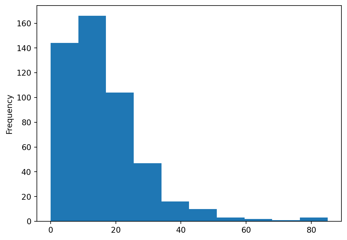

Assigning to _

pandas returns an object with the drawing from its plotting methods. Since you are in Jupyter environment, and you don’t need to work further with that object; you can assign it to _, a convention for an unused variable.

However, the default pandas plots can be a bit dull. A better option is to use another package, called seaborn.

import seaborn as sns

Why sns?

seaborn is, by convention, imported as sns. That came as a joke after Samuel Normal Seaborn, a fictional character The West Wing show.

The same plot using seaborn has a more pleasant default style and more customisability.

sns.displot(chicago_1918["influenza"])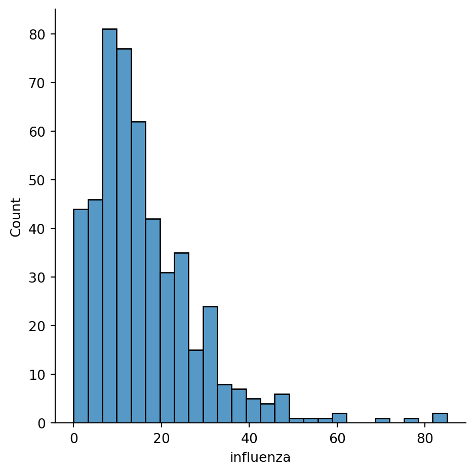

Histogram of influenza cases using `seaborn`

Note you are using sns instead of pd, as the function belongs to seaborn instead of pandas.

You can quickly see most of the areas have seen somewhere between 0 and 60 cases, approx. However, there are a few areas that have more, up to more than 80 cases.

Kernel Density Plots

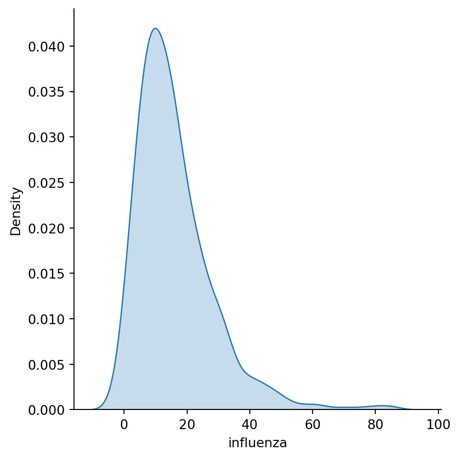
Histograms are useful, but they are artificial in the sense that a continuous variable is made discrete by turning the values into discrete groups. An alternative is kernel density estimation (KDE), which produces an empirical density function:

1sns.displot(chicago_1918["influenza"], kind="kde", fill=True)

1: kind="kde" specifies which type of a distribution plot should seaborn use and fill=True tells it to colour the area under the KDE curve.

Line and bar plots

Another very common way of visually displaying a variable is with a line or a bar chart. For example, if you want to generate a line plot of the (sorted) total cases by area:

_ = chicago_1918["influenza"].sort_values(ascending=False).plot()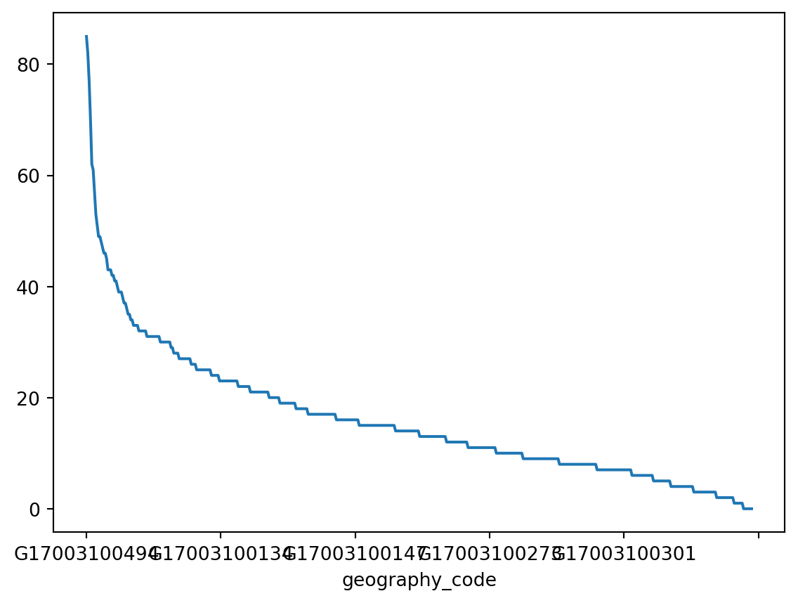

For a bar plot all you need to do is to change from plot to plot.bar. Since there are many census tracts, let us plot only the ten largest ones (which you can retrieve with head):

_ = chicago_1918["influenza"].sort_values(ascending=False).head(10).plot.bar()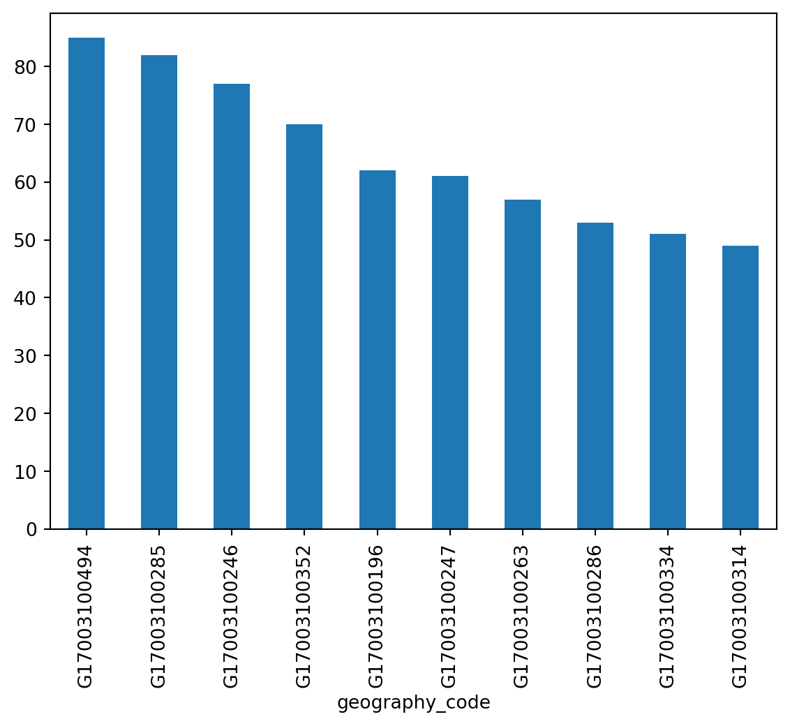

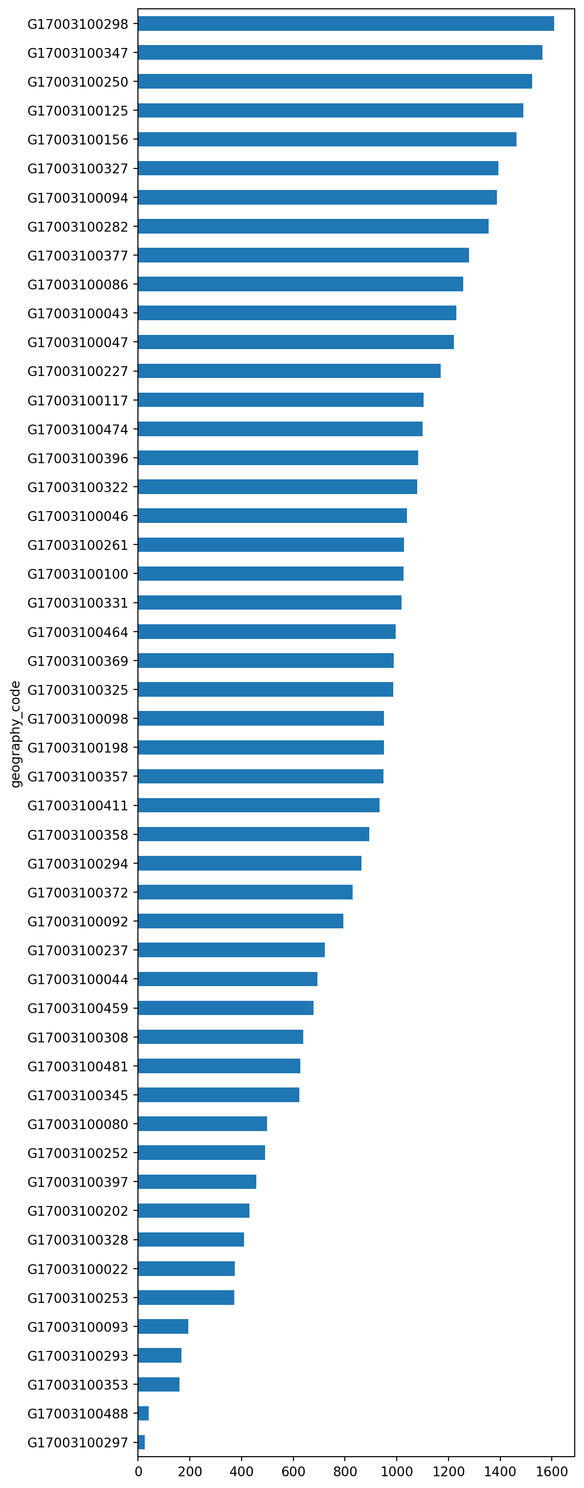
You can turn the plot around by displaying the bars horizontally (see how it’s just changing bar for barh). Let’s display now the top 50 areas and, to make it more readable, let us expand the plot’s height:

_ = (
    chicago_1918["total_population"]
    .sort_values()
    .head(50)
    .plot.barh(figsize=(6, 20))
)

Total cases by area as a horizontal bar plot

One line or multiple lines?

You may have noticed that in some cases, the code is on a single line, but longer code is split into multiple lines. Python requires you to follow the indentation rules, but apart from that, there are not a lot of other limits.

Tidy data

Caution

This section is a bit more advanced and hence considered optional. Feel free to skip it, move to the next, and return later when you feel more confident.

Once you can read your data in, explore specific cases, and have a first visual approach to the entire set, the next step can be preparing it for more sophisticated analysis. Maybe you are thinking of modeling it through regression, or on creating subgroups in the dataset with particular characteristics, or maybe you simply need to present summary measures that relate to a slightly different arrangement of the data than you have been presented with.

For all these cases, you first need what statistician, and general R wizard, Hadley Wickham calls “tidy data”. The general idea to “tidy” your data is to convert them from whatever structure they were handed in to you into one that allows convenient and standardized manipulation, and that supports directly inputting the data into what he calls “tidy” analysis tools. But, at a more practical level, what is exactly “tidy data”? In Wickham’s own words:

Tidy data is a standard way of mapping the meaning of a dataset to its structure. A dataset is messy or tidy depending on how rows, columns and tables are matched up with observations, variables and types.

He then goes on to list the three fundamental characteristics of “tidy data”:

Each variable forms a column.
Each observation forms a row.
Each type of observational unit forms a table.

If you are further interested in the concept of “tidy data”, I recommend you check out the original paper (open access) and the public repository associated with it.

Let us bring in the concept of “tidy data” to our own Chicago dataset. First, remember its structure:

chicago_1918.head()

	gross_acres	illit	unemployed_pct	ho_pct	agecat1	agecat2	agecat3	agecat4	agecat5	agecat6	agecat7	influenza	total_population	flu_rate
geography_code
G17003100001	1388.2	116	0.376950	0.124823	46	274	257	311	222	1122	587	9	2819	0.003193
G17003100002	217.7	14	0.399571	0.071647	35	320	441	624	276	1061	508	6	3265	0.001838
G17003100003	401.3	69	0.349558	0.092920	50	265	179	187	163	1020	392	8	2256	0.003546
G17003100004	86.9	11	0.422535	0.030072	43	241	129	141	123	1407	539	2	2623	0.000762
G17003100005	337.1	20	0.431822	0.084703	65	464	369	464	328	2625	1213	7	5528	0.001266

Thinking through tidy lenses, this is not a tidy dataset. It is not so for each of the three conditions:

Starting by the last one (each type of observational unit forms a table), this dataset actually contains not one but many observational units: the different areas of Chicago, captured by geography_code; and different observatoins for each area. To tidy up this aspect, you can create separate tables. You will probably want population groups divided by age as one tidy table and flu rates as another. Start by extracting relevant columns.

1influenza_rates = chicago_1918[["influenza"]]
influenza_rates.head()

1: You are not selecting a single columns with chicago_1918["influenza"] but a subset of columns. Just that the subset contains only one column, so you pass a list with a single column name as chicago_1918[["influenza"]]. Notice the double brackets.

	influenza
geography_code
G17003100001	9
G17003100002	6
G17003100003	8
G17003100004	2
G17003100005	7

population = chicago_1918.loc[:, "agecat1":"agecat7"]
population.head()

	agecat1	agecat2	agecat3	agecat4	agecat5	agecat6	agecat7
geography_code
G17003100001	46	274	257	311	222	1122	587
G17003100002	35	320	441	624	276	1061	508
G17003100003	50	265	179	187	163	1020	392
G17003100004	43	241	129	141	123	1407	539
G17003100005	65	464	369	464	328	2625	1213

At this point, the table influenza_rates is tidy: every row is an observation, every table is a variable, and there is only one observational unit in the table.

The other table (population), however, is not entirely tidied up yet: there is only one observational unit in the table, true; but every row is not an observation, and there are variable values as the names of columns (in other words, every column is not a variable). To obtain a fully tidy version of the table, you need to re-arrange it in a way that every row is an age category in an area, and there are three variables: geography_code, age category, and population count (or frequency).

Because this is actually a fairly common pattern, there is a direct way to solve it in pandas:

tidy_population = population.stack()
tidy_population.head()

geography_code         
G17003100001    agecat1     46
                agecat2    274
                agecat3    257
                agecat4    311
                agecat5    222
dtype: int64

The method stack, well, “stacks” the different columns into rows. This fixes our “tidiness” problems but the type of object that is returning is not a DataFrame:

type(tidy_population)

pandas.core.series.Series

It is a Series, which really is like a DataFrame, but with only one column. The additional information (geography_code and age category) are stored in what is called an multi-index. You will skip these for now, so you would really just want to get a DataFrame as you know it out of the Series. This is also one line of code away:

tidy_population_df = tidy_population.reset_index()
tidy_population_df.head()

	geography_code	level_1	0
0	G17003100001	agecat1	46
1	G17003100001	agecat2	274
2	G17003100001	agecat3	257
3	G17003100001	agecat4	311
4	G17003100001	agecat5	222

To which you can apply to renaming to make it look better:

tidy_population_df = tidy_population_df.rename(
    columns={"level_1": "age_category", 0: "count"}
)
tidy_population_df.head()

	geography_code	age_category	count
0	G17003100001	agecat1	46
1	G17003100001	agecat2	274
2	G17003100001	agecat3	257
3	G17003100001	agecat4	311
4	G17003100001	agecat5	222

Now our table is fully tidied up!

Grouping, transforming, aggregating

One of the advantage of tidy datasets is they allow to perform advanced transformations in a more direct way. One of the most common ones is what is called “group-by” operations. Originated in the world of databases, these operations allow you to group observations in a table by one of its labels, index, or category, and apply operations on the data group by group.

For example, given our tidy table with age categories, you might want to compute the total sum of the population by each category. This task can be split into two different ones:

Group the table in each of the different subgroups.
Compute the sum of count for each of them.

To do this in pandas, meet one of its workhorses, and also one of the reasons why the library has become so popular: the groupby operator.

pop_grouped = tidy_population_df.groupby("age_category")
pop_grouped

<pandas.core.groupby.generic.DataFrameGroupBy object at 0x7fa1fb4d3b90>

The object pop_grouped still hasn’t computed anything. It is only a convenient way of specifying the grouping. But this allows us then to perform a multitude of operations on it. For our example, the sum is calculated as follows:

1pop_grouped.sum(numeric_only=True)

1: You want a sum of numeric values, not strings. Try it with numeric_only=False to see the difference.

	count
age_category
agecat1	50776
agecat2	275363
agecat3	201654
agecat4	259954
agecat5	206358
agecat6	1171345
agecat7	522130

Similarly, you can also obtain a summary of each group:

pop_grouped.describe()

	count
	count	mean	std	min	25%	50%	75%	max
age_category
agecat1	496.0	102.370968	78.677423	0.0	46.75	82.0	136.00	427.0
agecat2	496.0	555.167339	423.526444	3.0	256.50	442.5	717.50	2512.0
agecat3	496.0	406.560484	301.564896	1.0	193.50	331.5	532.50	1917.0
agecat4	496.0	524.100806	369.875444	4.0	253.75	453.5	709.50	2665.0
agecat5	496.0	416.044355	281.825682	0.0	220.50	377.0	551.75	2454.0
agecat6	496.0	2361.582661	1545.469426	8.0	1169.75	2102.0	3191.75	9792.0
agecat7	496.0	1052.681452	722.955717	6.0	519.75	918.5	1379.25	4163.0

You will not get into it today as it goes beyond the basics this session wants to cover, but keep in mind that groupby allows you to not only call generic functions (like sum or describe), but also your own functions. This opens the door for virtually any kind of transformation and aggregation possible.

Additional reading

A good introduction to data manipulation in Python is Wes McKinney’s “Python for Data Analysis” (McKinney 2012).
To explore further some of the visualization capabilities in at your fingertips, the Python library seaborn is an excellent choice. Its online tutorial is a fantastic place to start.
A good extension is Hadley Wickham’s “Tidy data” paper (Wickham 2014), which presents a very popular way of organising tabular data for efficient manipulation.

Acknowledgements

This section is derived from A Course on Geographic Data Science by Arribas-Bel (2019), licensed under CC-BY-SA 4.0. The text was slightly adapted, mostly to accommodate a different dataset used.

References

Arribas-Bel, Dani. 2019. “A Course on Geographic Data Science.” The Journal of Open Source Education 2 (14). https://doi.org/10.21105/jose.00042.

Grantz, Kyra H, Madhura S Rane, Henrik Salje, Gregory E Glass, Stephen E Schachterle, and Derek AT Cummings. 2016. “Disparities in Influenza Mortality and Transmission Related to Sociodemographic Factors Within Chicago in the Pandemic of 1918.” Proceedings of the National Academy of Sciences 113 (48): 13839–44.

McKinney, Wes. 2012. Python for Data Analysis: Data Wrangling with Pandas, NumPy, and IPython. " O’Reilly Media, Inc.".

Wickham, Hadley. 2014. “Tidy Data.” Journal of Statistical Software 59 (10): 1–23. https://doi.org/10.18637/jss.v059.i10.

Footnotes

Data munging and data wrangling are used interchangeably. Pick the one you like.↩︎
Scalar is a single value, like a number (42) or a string ("towel").↩︎